データ処理,データベース,ディープラーニング分野のための基礎用語. 項目を 0-9,a-z, あーん,漢字順に並べている.
第三者のソフトウエア,データセット,製品等を説明しているものがあるが, それらの利用条件は利用者で確認すること.個々のソフトウエア,データセット,製品等の評価,評論は行わない.
【目次】
【サイト内の関連ページ】
参考 Web ページ:
2to3 は,Python バージョン 2 用のソースコードを Python バージョン 3 用に変換するプログラム.
詳しくは: 別ページで説明している.
顔のデータベース,顔の 68 ランドマークが付いている.
C. Sagonas, G. Tzimiropoulos, S. Zafeiriou and M. Pantic, "300 Faces in-the-Wild Challenge: The First Facial Landmark Localization Challenge," 2013 IEEE International Conference on Computer Vision Workshops, 2013, pp. 397-403, doi: 10.1109/ICCVW.2013.59.
https://ibug.doc.ic.ac.uk/media/uploads/documents/sagonas_2016_imavis.pd
【関連項目】 HELEN データセット, iBUG 300-W データセット, face alignment, 顔ランドマーク (facial landmark)の検出, 3次元の顔の再構成 (3D face reconstruction), OpenMMLab, 顔の 68 ランドマーク, 顔のデータベース
3DF Zephyr Free は,フォトグラメトリのソフトウエア 3dF Zephyr の無料版
【関連項目】 フォトグラメトリ, Meshroom
3DDFA_V2 は, 3次元の顔の再構成 (3D face reconstruction) のうち dense vertices regression を行う一手法.論文は,2020年発表.
Jianzhu Guo, Xiangyu Zhu, Yang Yang, Fan Yang, Zhen Lei, Stan Z. Li, Towards Fast, Accurate and Stable 3D Dense Face Alignment, ECCV 2020.
Gradio での 3DDFA_V2 のオンライン実行
URL: https://github.com/cleardusk/3DDFA_V2
作成された3次元モデルを Blender にインポートした画面.
次のページは,Google Colaboratory のページである.ページを開き実行できる.
URL: https://colab.research.google.com/drive/1OKciI0ETCpWdRjP-VOGpBulDJojYfgWv [Google Colaboratory]
実行により,3次元のポリゴンが得られていることを確認できる.
結果は /content/3DDFA_V2/examples/results/ にできる. ここには,顔の3次元データであるポリゴンメッシュ(.obj ファイル)もある.
.obj ファイルをダウンロードし Blender で表示してみると次のようになる.
画像から,物体検出を行うとともに,その3次元の向きの推定も行う.
【関連項目】 Objectron
3次元ゲームエンジン (3-D game engine) の機能を持つソフトウエアとしては, GoDot, Open 3D Engine, Unreal Engine, Panda3D などがある.
3次元の顔の再構成 (3D face reconstruction) は, 顔の写った画像から,元の顔の3次元の形を構成すること.
3次元の顔の再構成は,次の2つの種類がある.
3次元再構成 (3D reconstruction) の機能をもつソフトウエアとしては, colmap, Meshroom がある.
【関連項目】 colmap, Meshroom, Multi View Stereo, OpenMVG, OpenMVS, Structure from Motion
3次元点群データ (3-D point cloud data) を扱うには,MeshLab や CloudCompare が便利である.
7-Zip は,Windows で動くソフトウエア.ファイルの圧縮や展開の機能を持つ.
7-Zip のURL: https://sevenzip.osdn.jp/
7-Zip のインストールの詳細: 別ページで説明している
URL: https://www.visuallocalization.net/datasets/
M.Zeiler の AdaDelta 法は,学習率をダイナミックに変化させる技術. 学習率をダイナミックに変化させる技術は,その他 Adam 法なども知られる.
確率的勾配降下法 (SGD 法) をベースとしているが, 確率的勾配降下法が良いのか,Adadelta 法が良いのかは,一概には言えない.
【Keras のプログラム】
from tensorflow.keras.optimizers import Adadelta
optimizer = Adadelta(rh=0.95)
M. Zeiler, Adadelta An adaptive learning rate method, 2012.
Adam 法は,学習率をダイナミックに変化させる技術. 学習率をダイナミックに変化させる技術は,その他 AdaDelta 法なども知られる. Adam 法を使うプログラム例は次の通り.
【Keras のプログラム】
m.compile(
    optimizer=tf.keras.optimizers.Adam(learning_rate=0.001),
    loss='sparse_categorical_crossentropy',
    metrics=['sparse_categorical_crossentropy', 'accuracy']
)
Diederik Kingma and Jimmy Ba, Adam: A Method for Stochastic Optimization, 2014, CoRR, abs/1412.6980
ADE20K データセット は, セマンティック・セグメンテーション,シーン解析(scene parsing), インスタンス・セグメンテーション (instance segmentation)についてのアノテーション済みの画像データセットである.
次の特色がある
画像数,オブジェクト数などは次の通り.
うち学習用: 25,574 枚, うち検証用: 2,000 枚, うちテスト用: 3,000 枚.
利用には,次の URL で登録が必要.
ADE20K データセットの URL: http://groups.csail.mit.edu/vision/datasets/ADE20K/
【関連情報】
Bolei Zhou, Hang Zhao, Xavier Puig, Sanja Fidler, Adela Barriuso, Antonio Torralba, Scene Parsing Through ADE20K Dataset, CVPR 2017, also CoRR, abs/1608.05442, 2017.
Bolei Zhou, Hang Zhao, Xavier Puig, Tete Xiao, Sanja Fidler, Adela Barriuso and Antonio Torralba, Semantic Understanding of Scenes through ADE20K Dataset, International Journal on Computer Vision (IJCV), also CoRR, https://arxiv.org/pdf/1608.05442v2.pdf
このスターターコードは,画像1枚について元画像とアノテーションを表示するもの
【関連項目】 semantic segmentation, シーン解析(scene parsing), インスタンス・セグメンテーション (instance segmentation), Detectron2 CASILVision, MIT Scene Parsing Benchmark, 物体検出
AFLW (Annotated Facial Landmarks in the Wild) データセットは, Flickr から収集された24,386枚の顔画像である. さまざまな表情,民族,年齢,性別,撮影条件,環境条件の顔が収集されている. それぞれの顔には,最大21個の顔ランドマークが付けられている.
次の URL で公開されているデータセット(オープンデータ)である.
URL: https://www.tugraz.at/institute/icg/research/team-bischof/lrs/downloads/aflw/
【関連情報】
M. Köstinger, P. Wohlhart, P. M. Roth and H. Bischof, "Annotated Facial Landmarks in the Wild: A large-scale, real-world database for facial landmark localization," 2011 IEEE International Conference on Computer Vision Workshops (ICCV Workshops), 2011, pp. 2144-2151, doi: 10.1109/ICCVW.2011.6130513.
https://github.com/open-mmlab/mmpose/blob/master/docs/en/tasks/2d_face_keypoint.md#aflw-dataset
Python 処理系, conda その他の詰め合わせ. パッケージ管理は anaconda, conda コマンドで行う. pip や python setpy.py でのインストール予定がない場合には候補の1つになりえる.
Windows での Anaconda3 のインストールには,複数の方法がある.次のいずれかによりインストールできる.
winget をインストールしたのち,コマンドプロンプトを管理者として実行し,「winget install Anaconda3」を実行.
【関連項目】 Python のインストール
手作業で収集された,「in-the-wild」の顔と年齢のデータベース. 年号まで正確に記録された顔画像が含まれている.
次の URL で公開されているデータセット(オープンデータ)である.
https://ibug.doc.ic.ac.uk/resources/agedb/
S. Moschoglou, A. Papaioannou, C. Sagonas, J. Deng, I. Kotsia and S. Zafeiriou, "AgeDB: The First Manually Collected, In-the-Wild Age Database," 2017 IEEE Conference on Computer Vision and Pattern Recognition Workshops (CVPRW), 2017, pp. 1997-2005, doi: 10.1109/CVPRW.2017.250.
【関連項目】 顔認識 (face recognition), 顔のデータベース
image matting のデータセット. 3種類の前景(Salient Opaque, Salient Transparent/Meticulous, Non-Salient)を含む 500枚の画像について,元画像と alpha matte と Trimap のデータセットである.
次の URL で公開されているデータセット(オープンデータ)である.
URL: https://drive.google.com/drive/folders/1IyPiYJUp-KtOoa-Hsm922VU3aCcidjjz
Jizhizi Li, Jing Zhang, DaCheng Tao, Deep Automatic Natural Image Matting, CoRR, abs/2107.07235v1, 2021.
【関連用語】 image matting, オープンデータ (open data)
AlexeyAB darknet は,YOLOv3, YOLOv4 の機能などを持つ.
Alexey による darknet の実装(GitHub)ページ: https://github.com/AlexeyAB/darknet
AlexNet の場合
input 3@224x224
conv 11x11
  96@55x55
pooling
conv 5x5
  256@27x27
pooling
  16@5x5
conv 3x3
  384@13x13
conv 3x3
  384@13xx13
conv 3x3
  256@13x13
affine
  4096
affine
  4096
  1000
参考文献: ch08/deep=cnvnet.py
機械学習による物体検出では, 「AP」は,「average precision」の意味である.
「Applications of Deep Neural Networks」は,ディープラーニングに関するテキスト. ニューラルネットワーク, CNN (convolutional neural network), LSTM (Long Short-Term Memory), GRU (Gated Recurrent Neural Networks), GAN (Generative Adversarial Network), 強化学習とその応用について学ぶことができる. Python, TensorFlow, Keras を使用している.
【関連項目】 CNN (convolutional neural network), GAN (Generative Adversarial Network), GRU (Gated Recurrent Neural Networks), Keras, LSTM (Long Short-Term Memory), TensorFlow, ディープラーニング ニューラルネットワーク, 強化学習
距離学習の1手法である. 分類モデルが特徴ベクトルを生成するための複数の層と,最終層の softmax から構成されているとき, その分類モデルでの,特徴ベクトルを生成するための複数の層の出力に対して, L2 正規化の処理と,Angular Magin Penalty 層による処理を追加し,softmax 層につなげる.
deepface, InsightFace などで実装されている.
【関連項目】 deepface, InsightFace, 顔検証 (face verification), 顔識別 (face identification), 顔認識 (face recognition), 顔に関する処理
BASNet は, ディープラーニングにより,Salient Object Detection (顕著なオブジェクトの検出)を行う一手法.2019年発表.
BASNet は次の2つのモジュールから構成される.
入力画像から saliency map を生成する. U-Net に類似の構造を持つ,教師有りの Encoder-Decoder ネットワークである. この段階での saliency map は,粗い (coarse) ものである.
Predict Module が生成した saliency map をリファイン (refine) する. Residual Refinement Module は Predict Module が生成した saliency map と,正解 (ground truth) との残差 (residuals) を学習する.
Salient Object Detection は, 視覚特性の異なるオブジェクトを,画素単位で切り出す. 前景と背景の分離に役立つ場合がある.人間がマスクの指定や塗り分け(Trimap など)を行うことはない.
元画像
BASNet 法の結果
Qin, Xuebin and Zhang, Zichen and Huang, Chenyang and Gao, Chao and Dehghan, Masood and Jagersand, Martin, BASNet: Boundary-Aware Salient Object Detection, The IEEE Conference on Computer Vision and Pattern Recognition (CVPR), 2019
【関連用語】 U-Net, salient object detection, semantic segmentation,
次のコマンドやプログラムは Google Colaboratory で動く(コードセルを作り,実行する).
BASNet のテストプログラムのオンライン実行を行うまでの手順を示す.
!git clone https://github.com/NathanUA/BASNet.git
公式ページ https://github.com/xuebinqin/BASNet の指示による. 学習済みモデル(ファイル名 basenet.pth)は,次で公開されている. ダウンロードし,saved_models/basnet_bsi の下に置く
https://drive.google.com/open?id=1s52ek_4YTDRt_EOkx1FS53u-vJa0c4nu
%cd PyTorch-UNet
!curl -L https://github.com/opencv/opencv/blob/master/samples/data/fruits.jpg?raw=true -o fruits.jpg
!curl -L https://github.com/opencv/opencv/blob/master/samples/data/home.jpg?raw=true -o home.jpg
!curl -L https://github.com/opencv/opencv/blob/master/samples/data/squirrel_cls.jpg?raw=true -o squirrel_cls.jpg
from IPython.display import Image, display
display(Image('fruits.jpg'))
display(Image('home.jpg'))
display(Image('squirrel_cls.jpg'))
%cd BASNet
!python basnet_test.py
【関連項目】 Residual Networks (ResNets)
BioID 顔データベースは,23名, 1521枚のモノクロの画像.解像度は 384x286 である.目の位置に関するデータを含む.
BioID 顔データベースは次の URL で公開されているデータセット(オープンデータ)である.
Blenderは,3次元コンピュータグラフィックス・アニメーションソフトウエアである. 3次元モデルの編集,レンダリング,光源やカメラ等を設定しての3次元コンピュータグラフィックス・アニメーション作成機能がある.
【関連項目】 bpy (blenderpy), yuki-koyama の blender-cli-rendering
Windows での Blender のインストールは,複数の方法がある.
Ubuntu での Blender のインストールは,別ページで説明している.
次の動画は,Blender のモーショントラッキング機能を用いた映像作成について説明している.
https://www.youtube.com/watch?v=lY8Ol2n4o4A
次の動画は,作成された映像,グリーンバックの映像である.
https://www.youtube.com/watch?v=FFJ_THGj72U
bpy (blenderpy) では,Blender がPython モジュールになっている.
【関連項目】 Blender yuki-koyama の blender-cli-rendering
PyPI を用いてのインストールでは,2021年12月時点では,使用する Python はバージョン 3.7,Blender は 2.8. 新しい Blender の Python モジュールを必要する場合には,下の項目を見ること.
https://pypi.org/project/bpy/ の記載により,PyPI の bpy (blenderpy) のインストールを行う.
「-3.7」のところには, いま確認した Python のバージョンを指定する.
「-3.7」のところには, いま確認した Python のバージョンを指定する.
エラーメッセージが出ていなければ OK.
詳しくは,別ページで説明している.
C++ ビルドツール (Build Tools) のインストール, Git のインストール, cmake のインストール, svn のインストール, NVIDIA CUDA ツールキット,NVIDIA cuDNN のインストールを行うこと. が必要.
インストールしたい Blender のバージョンにあうタグを,次のページで探す.
「v3.0.0」のところには,使用したいバージョンの Blender のタグを指定すること.
mkdir c:\tools
cd c:\tools
rmdir /s /q blender
git clone -b v3.0.0 https://github.com/blender/blender
終了まで時間がかかるので,しばらく待つ
cd c:\tools
cd blender
make update 2019b
make release 2019b
cd c:\tools
cd blender
rmdir /s /q build
mkdir build
cd build
cmake -G "Visual Studio 16 2019" -A x64 -T host=x64 -DWITH_PYTHON_INSTALL=OFF -DWITH_PYTHON_MODULE=ON ..
cmake --build . --config RELEASE --target INSTALL
「c:\Program Files\Python39」のところは, Python のインストールディレクトリを指定すること.
python -m pip install numpy
cd c:\tools\blender\build\release
copy bin\bpy.pyd c:\Program Files\Python39\Lib\site-packages\
copy bin\*.dll c:\Program Files\Python39\Lib\site-packages\
del c:\Program Files\Python39\Lib\site-packages\python36.dll
xcopy /E bin\3.0 c:\Program Files\Python39\
コマンドプロンプトで次のコマンドを実行.
エラーメッセージが出なければ OK.
python -c "import bpy; scene = bpy.data.scenes['Scene']; print(scene)"
Boost は, C++ のライブラリ.
Boost の URL: https://www.boost.org/
C++ ビルドツール (Build Tools) のインストール, Git のインストール, Python のインストール が必要.
C:\Program Files\boost 下にインストールするものとして説明する.
コマンドプロンプトを管理者として実行し,次のコマンドを実行.
cd "c:\Program Files"
rmdir /s /q boost
git clone --recursive https://github.com/boostorg/boost
cd boost
.\bootstrap.bat
.\b2.exe --prefix=build --build-type=complete toolset=msvc link=static,shared address-model=64 install
次のコマンドで確認する.ここで確認したことは,のちほど,使用する.
dir "C:\Program Files\boost\build\include"
Windows での環境変数の設定は,マイコンピュータを右クリック → プロパティ→ 詳細設定 → 環境変数をクリック
Windowsの画面の表示では、「\」(円マーク)が表示される
次のように設定する.今までの操作で「--prefix」のところに指定してきたディレクトリに一致させること.
C:\Program Files\boost\build
次のように設定する.
C:\Program Files\boost\build\lib
C:\Program Files\boost\build\lib
「boost-1_78」のところは,先ほど確認したインクルードディレクトリに一致させること.
C:\Program Files\boost\build\include\boost-1_78
Visual Studio の x64 Native Tools コマンドプロンプトを管理者として実行する. 次のコマンドを実行する.
「boost-1_78」のところは,先ほど確認したインクルードディレクトリに一致させること.
cl /EHsc /I "C:\Program Files\boost\build\include\boost-1_78" ^
    "C:\Program Files\boost\libs\geometry\example\01_point_example.cpp"
.\01_point_example.exe
Ubuntu でインストールを行うには,端末で,次のコマンドを実行する.
sudo apt -y update
sudo apt -y install libboost-all-dev
Boston housing price 回帰データセットは,次のプログラムでロードできる.
【Keras のプログラム】
from tensorflow.keras.datasets import boston_housing
(x_train, y_train), (x_test, y_test) = boston_housing.load_data()
【関連項目】 Keras に付属のデータセット
ディープラーニングによる物体検出のための学習と検証では, アノテーションとして,物体のバウンディングボックスが広く用いられている.
ディープラーニングによるインスタンス・セグメンテーション (instance segmentation)でも, Tian らの BoxInst (2021年発表) のように,画素単位でのアノテーションでなく, バウンディングボックスを用いる手法が登場している.
【関連項目】 インスタンス・セグメンテーション (instance segmentation), バウンディングボックス, 物体検出,
正しくマスクが装着された状態の顔の写真 (CMFD) と, 正しくマスクが装着されていない状態の顔の写真 (IMFD) のデータセット.
Adnane Cabani and Karim Hammoudi and Halim Benhabiles and Mahmoud Melkemi, MaskedFace-Net -- A Dataset of Correctly/Incorrectly Masked Face Images in the Context of COVID-19, Smart Health, 2020.
【関連項目】 顔のデータベース, 顔検出 (face detection)
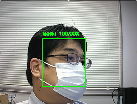
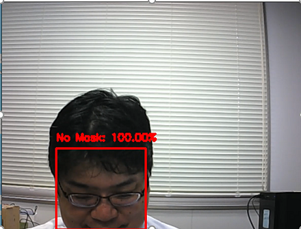
Chandrika Deb の顔マスク検出 (Chandrika Deb's Face Mask Detection) により, マスク有りの画像とマスク無しの画像を用いて,ディープラーニングによる学習を行い, その後,マスク有りの顔と,マスク無しの顔を検出.
次の2種類のデータを用いて学習を行い,マスク有りの顔と,マスク無しの顔を検出.
コマンドプロンプトを管理者として実行し,次のコマンドを実行.
mkdir c:\pytools
cd c:\pytools
rmdir /s /q Face-Mask-Detection
git clone https://github.com/chandrikadeb7/Face-Mask-Detection
cd Face-Mask-Detection
python -m pip install -U -r requirements.txt
CMFD.zip をダウンロードしたとして説明を続ける.
CMFD.zip を展開(解凍).中の画像ファイルを選び,c:\pytools\Face-Mask-Detection\dataset\with_mask にコピーする
source ~/a/bin/activate
cd c:\pytools\Face-Mask-Detection
python train_mask_detector.py --dataset dataset
python detect_mask_image.py --image images/pic1.jpeg
python detect_mask_video.py
結果のビデオファイル: ../db/1.mp4
Caffe 2 のインストール
参考 Web ページ
Caltech Pedestrian データセット は,都市部を走行中の車両から撮影したデータ. 機械学習による物体検出 の学習や検証に利用できるデータセットである.
Caltech Pedestrian データセットは次の URL で公開されているデータセット(オープンデータ)である.
URL: http://www.vision.caltech.edu/Image_Datasets/CaltechPedestrians/
【関連情報】
Large-scale CelebFaces Attributes (CelebA) データセットは,顔画像とアノテーションのデータ. 機械学習による顔検出,顔ランドマーク (facial landmark),顔認識,顔の生成などの学習や検証に利用できるデータセットである.
Large-scale CelebFaces Attributes (CelebA) データセットは次の URL で公開されているデータセット(オープンデータ)である.
URL: https://mmlab.ie.cuhk.edu.hk/projects/CelebA.html
【関連情報】
Deep Learning Face Attributes in the Wild, Ziwei Liu, Ping Luo, Xiaogang Wang, Xiaoou Tang, ICCV 2015.
【関連項目】 顔のデータベース, 顔ランドマーク (facial landmark)
CityGML は,3次元の都市,3次元の景観を扱う機能を持つデータフォーマット. 次のようなモジュールがある.
Appearance, Bridge, Building, CityFurniture, LandUse, Relief, Transportation, Tunnel, Vegetation, Vegetation, WaterBody, TexturedSurface
CityGML の公式情報は,Open Geospatial Consortium のページで公開されている.
Open Geospatial Consortium の CityGML ページ: https://www.ogc.org/standards/citygml
CityGML の仕様書も,このページで公開されている.
CityGML のビューワには FZKViewer がある. Windows での FZKViewer のインストールは 別ページで説明している.
【関連項目】 FZKViewer
CSAILVision の公式デモ(GitHub のページ): https://colab.research.google.com/github/CSAILVision/semantic-segmentation-pytorch/blob/master/notebooks/DemoSegmenter.ip
CGAL のインストールは,複数の方法がある. ここでは, vcpkg を使う方法を説明する.
c:\vcpkg\vcpkg search cgal
c:\vcpkg\vcpkg install cgal[qt]:x64-windows
c:\vcpkg\installed\x64-windows\bin
Ubuntu でインストールを行うには,端末で,次のコマンドを実行する.
sudo apt -y update
sudo apt -y install libcgal-dev libcgal-qt5-dev
写真やビデオから,マスクありの顔と,マスク無しの顔を検出する技術およびソフトウエア. 顔検出,マスク有りの顔とマスク無しの顔の分類を同時に行っている. MobileNetV2 (ディープニューラルネットワーク)を使用.
Bing Search API, Kaggle dataset, RMDF dataset から収集された顔のデータセット(マスクあり: 2165 枚,マスクなし 1930 枚)が同封.
ソースコードは公開されており,画像を追加して学習をやり直すことも可能
URL: Chandrika Deb, https://github.com/chandrikadeb7/Face-Mask-Detection
【関連項目】 cabani の MaskedFace-Net データセット, Face Mask Detection, マスク付き顔の処理 顔検出 (face detection)
次のコマンドやプログラムは Google Colaboratory で動く(コードセルを作り,実行する).
!rm -rf Face-Mask-Detection
!git clone https://github.com/chandrikadeb7/Face-Mask-Detection
%cd Face-Mask-Detection
!pip3 install -U -r requirements.txt
Chandrika Deb の顔マスク検出に同封のデータセット(Deb Bing Search API, Kaggle dataset, RMDF dataset から収集された顔のデータセット(マスクあり: 2165 枚,マスクなし 1930 枚)により学習を行う.
!python3 train_mask_detector.py --dataset dataset
!sed -i -e 's/cv2.imshow("Output", image)/cv2.imwrite("result.png", image)/g' detect_mask_image.py
!sed -i -e 's/cv2.waitKey(0)//g' detect_mask_image.py
!python3 detect_mask_image.py --image images/pic1.jpeg
from IPython.display import Image, display
display(Image('result.png'))
curl は URL を指定して画像ファイルをダウンロードしている.
!curl -O https://www.kkaneko.jp/sample/face/3284.png
!python3 detect_mask_image.py --image 3284.png
from IPython.display import Image, display
display(Image('result.png'))
!curl -O https://www.kkaneko.jp/sample/face/3288.png
!python3 detect_mask_image.py --image 3288.png
from IPython.display import Image, display
display(Image('result.png'))
mkdir c:\pytools
cd c:\pytools
rmdir /s /q Face-Mask-Detection
git clone --recursive https://github.com/chandrikadeb7/Face-Mask-Detection
cd Face-Mask-Detection
python -m pip install -U -r requirements.txt
Chandrika Deb の顔マスク検出に同封のデータセット(Deb Bing Search API, Kaggle dataset, RMDF dataset から収集された顔のデータセット(マスクあり: 2165 枚,マスクなし 1930 枚)により学習を行う. その後,顔マスク検出を行う.
cd c:\pytools\Face-Mask-Detection
python train_mask_detector.py --dataset dataset
「python detect_mask_video.py 」はカメラの顔マスク検出を行う.
cd c:\pytools\Face-Mask-Detection
python detect_mask_image.py --image images/pic1.jpeg
python detect_mask_video.py
結果のビデオファイル: ../db/2.mp4
TensorFlow で,GPU のメモリ不足でエラーメッセージがでて,プログラムが止まる場合, プログラムの先頭部分に次を追加すると解決する場合がある.
メッセージ
Internal: Attempting to perform BLAS operation using StreamExecutor without BLAS support
解決策:Python プログラムの先頭部分に次を追加すると解決する場合がある.
import tensorflow as tf
gpus = tf.config.experimental.list_physical_devices('GPU')
tf.config.experimental.set_memory_growth(gpus[0], True)
前準備:事前に Python のインストール, NVIDIA CUDA ツールキット,NVIDIA cuDNN のインストールを行うこと.
sudo apt -y update
sudo apt -y install git
cd /usr/local
sudo rm -rf Face-Mask-Detection
sudo git clone https://github.com/chandrikadeb7/Face-Mask-Detection
sudo chown -R $USER Face-Mask-Detection
# システム Python の環境とは別の Python の隔離された環境(システム Python を使用)を作成
sudo apt -y update
sudo apt -y install python3-venv
python3 -m venv ~/a
source ~/a/bin/activate
cd /usr/local/Face-Mask-Detection
pip install -U -r requirements.txt
pip list
Chandrika Deb の顔マスク検出に同封のデータセット(Deb Bing Search API, Kaggle dataset, RMDF dataset から収集された顔のデータセット(マスクあり: 2165 枚,マスクなし 1930 枚)により学習を行う. その後,顔マスク検出を行う.
source ~/a/bin/activate
cd /usr/local/Face-Mask-Detection
python train_mask_detector.py --dataset dataset
「python detect_mask_video.py 」はカメラの顔マスク検出を行う.
python detect_mask_image.py --image images/pic1.jpeg
python detect_mask_video.py
CIFAR-10 データセット(Canadian Institute for Advanced Research, 10 classes) は,クラス数 10 の カラー画像と,各画像に付いたのラベルから構成されるデータセットである. 機械学習での画像分類の学習や検証に利用できる.
(内訳)60000枚の内訳は次の通りである
50000枚:教師データ
10000枚:検証データ
CIFAR-10 データセットは次の URL で公開されているデータセット(オープンデータ)である.
CIFAR-10 データセットの URL: https://www.cs.toronto.edu/~kriz/cifar.html
【関連情報】
【関連項目】 CIFAR-100 データセット(Canadian Institute for Advanced Research, 100 classes), Keras に付属のデータセット, TensorFlow データセット, オープンデータ, 画像分類
次の Python プログラムは,TensorFlow データセットから,CIFAR-10 データセットのロードを行う. x_train, y_train が学習用のデータ.x_test, y_test が検証用のデータになる.
次のプログラムでは、x_train と y_train を 25枚分表示することにより,x_train と y_train が,画像であることが確認できる.
tensorflow_datasets の loadで, 「batch_size = -1」を指定して,一括読み込みを行っている.
from __future__ import absolute_import, division, print_function, unicode_literals
import tensorflow.compat.v2 as tf
tf.enable_v2_behavior()
print(tf.__version__)
import numpy as np
import tensorflow_datasets as tfds
%matplotlib inline
import matplotlib.pyplot as plt
import warnings
warnings.filterwarnings('ignore')   # Suppress Matplotlib warnings
%matplotlib inline
import matplotlib.pyplot as plt
import warnings
warnings.filterwarnings('ignore')   # Suppress Matplotlib warnings
# CIFAR-10 データセットのロード
cifar10, cifar10_metadata = tfds.load('cifar10', with_info = True, shuffle_files=True, as_supervised=True, batch_size = -1)
x_train, y_train, x_test, y_test = cifar10['train'][0], cifar10['train'][1], cifar10['test'][0], cifar10['test'][1]
plt.style.use('default')
plt.figure(figsize=(10,10))
for i in range(25):
    plt.subplot(5,5,i+1)
    plt.xticks([])
    plt.yticks([])
    plt.grid(False)
# squeeze は,サイズ1の次元を削除.numpy は tf.Tensor を numpy に変換
    plt.imshow(np.squeeze(x_train[i]), cmap=plt.cm.binary)
    plt.xlabel(y_train[i].numpy())
# 確認表示
plt.show()
次の Python プログラムは,Keras に付属のデータセットの中にある CIFAR-10 データセットのロードを行う. x_train, y_train が学習用のデータ.x_test, y_test が検証用のデータになる.
次のプログラムでは,x_train と y_train を 25枚分表示することにより,x_train と y_train が,カラー画像であることが確認できる.
import tensorflow.keras
from tensorflow.keras.datasets import cifar10
%matplotlib inline
import matplotlib.pyplot as plt
import warnings
warnings.filterwarnings('ignore')   # Suppress Matplotlib warnings
# CIFAR-10 データセットのロード
(x_train, y_train), (x_test, y_test) = cifar10.load_data()
plt.style.use('default')
plt.figure(figsize=(10,10))
for i in range(25):
    plt.subplot(5,5,i+1)
    plt.xticks([])
    plt.yticks([])
    plt.grid(False)
    plt.imshow(x_train[i], cmap=plt.cm.binary)
    plt.xlabel(y_train[i])
# 確認表示
plt.show()
次の Python プログラムは,TensorFlow データセットから,CIFAR-10 データセットのロードを行う. x_train, y_train が学習用のデータ.x_test, y_test が検証用のデータになる.
次のプログラムでは、x_train と y_train を 25枚分表示することにより,x_train と y_train が,画像であることが確認できる.
tensorflow_datasets の loadで, 「batch_size = -1」を指定して,一括読み込みを行っている.
ロードの後,正規化を行う.type は型,shape はサイズ,np.max と np.mi は最大値と最小値.
from __future__ import absolute_import, division, print_function, unicode_literals
import tensorflow.compat.v2 as tf
tf.enable_v2_behavior()
print(tf.__version__)
import numpy as np
import tensorflow_datasets as tfds
%matplotlib inline
import matplotlib.pyplot as plt
import warnings
warnings.filterwarnings('ignore')   # Suppress Matplotlib warnings
%matplotlib inline
import matplotlib.pyplot as plt
import warnings
warnings.filterwarnings('ignore')   # Suppress Matplotlib warnings
# CIFAR-10 データセットのロード
cifar10, cifar10_metadata = tfds.load('cifar10', with_info = True, shuffle_files=True, as_supervised=True, batch_size = -1)
x_train, y_train, x_test, y_test = cifar10['train'][0], cifar10['train'][1], cifar10['test'][0], cifar10['test'][1]
plt.style.use('default')
plt.figure(figsize=(10,10))
for i in range(25):
    plt.subplot(5,5,i+1)
    plt.xticks([])
    plt.yticks([])
    plt.grid(False)
# squeeze は,サイズ1の次元を削除.numpy は tf.Tensor を numpy に変換
    plt.imshow(np.squeeze(x_train[i]), cmap=plt.cm.binary)
    plt.xlabel(y_train[i].numpy())
# 確認表示
plt.show()
# メタデータの表示
print(cifar10_metadata)
# 正規化
# 【x_train, x_test, y_train, y_test の numpy ndarray への変換と,値の範囲の調整(値の範囲が 0 〜 255 であるのを,0 〜 1 に調整)】
x_train = x_train.numpy().astype("float32") / 255.0
x_test = x_test.numpy().astype("float32") / 255.0
y_train = y_train.numpy()
y_test = y_test.numpy()
print(type(x_train), x_train.shape, np.max(x_train), np.min(x_train))
print(type(x_test), x_test.shape, np.max(x_test), np.min(x_test))
print(type(y_train), y_train.shape, np.max(y_train), np.min(y_train))
print(type(y_test), y_test.shape, np.max(y_test), np.min(y_test))
CIFAR-100 データセット(Canadian Institute for Advanced Research, 100 classes) は,機械学習での画像分類の学習や検証に利用できるデータセット.
CIFAR-100 データセットは次の URL で公開されているデータセット(オープンデータ)である.
https://www.cs.toronto.edu/~kriz/cifar.html
【関連情報】
【関連項目】 CIFAR-10 データセット(Canadian Institute for Advanced Research, 10 classes), Keras に付属のデータセット, TensorFlow データセット, オープンデータ, 画像分類
次の Python プログラムは,TensorFlow データセットから,CIFAR-100 データセットのロードを行う. x_train, y_train が学習用のデータ.x_test, y_test が検証用のデータになる.
次のプログラムでは、x_train と y_train を 25枚分表示することにより,x_train と y_train が,画像であることが確認できる.
tensorflow_datasets の loadで, 「batch_size = -1」を指定して,一括読み込みを行っている.
from __future__ import absolute_import, division, print_function, unicode_literals
import tensorflow.compat.v2 as tf
tf.enable_v2_behavior()
print(tf.__version__)
import numpy as np
import tensorflow_datasets as tfds
%matplotlib inline
import matplotlib.pyplot as plt
import warnings
warnings.filterwarnings('ignore')   # Suppress Matplotlib warnings
%matplotlib inline
import matplotlib.pyplot as plt
import warnings
warnings.filterwarnings('ignore')   # Suppress Matplotlib warnings
# CIFAR-100 データセットのロード
cifar100, cifar100_metadata = tfds.load('cifar100', with_info = True, shuffle_files=True, as_supervised=True, batch_size = -1)
x_train, y_train, x_test, y_test = cifar100['train'][0], cifar100['train'][1], cifar100['test'][0], cifar100['test'][1]
plt.style.use('default')
plt.figure(figsize=(10,10))
for i in range(25):
    plt.subplot(5,5,i+1)
    plt.xticks([])
    plt.yticks([])
    plt.grid(False)
# squeeze は,サイズ1の次元を削除.numpy は tf.Tensor を numpy に変換
    plt.imshow(np.squeeze(x_train[i]), cmap=plt.cm.binary)
    plt.xlabel(y_train[i].numpy())
# 確認表示
plt.show()
次の Python プログラムは,TensorFlow データセットから,CIFAR-100 データセットのロードを行う. x_train, y_train が学習用のデータ.x_test, y_test が検証用のデータになる.
次のプログラムでは、x_train と y_train を 25枚分表示することにより,x_train と y_train が,画像であることが確認できる.
tensorflow_datasets の loadで, 「batch_size = -1」を指定して,一括読み込みを行っている.
ロードの後,正規化を行う.type は型,shape はサイズ,np.max と np.mi は最大値と最小値.
from __future__ import absolute_import, division, print_function, unicode_literals
import tensorflow.compat.v2 as tf
tf.enable_v2_behavior()
print(tf.__version__)
import numpy as np
import tensorflow_datasets as tfds
%matplotlib inline
import matplotlib.pyplot as plt
import warnings
warnings.filterwarnings('ignore')   # Suppress Matplotlib warnings
%matplotlib inline
import matplotlib.pyplot as plt
import warnings
warnings.filterwarnings('ignore')   # Suppress Matplotlib warnings
# CIFAR-100 データセットのロード
cifar100, cifar100_metadata = tfds.load('cifar100', with_info = True, shuffle_files=True, as_supervised=True, batch_size = -1)
x_train, y_train, x_test, y_test = cifar100['train'][0], cifar100['train'][1], cifar100['test'][0], cifar100['test'][1]
plt.style.use('default')
plt.figure(figsize=(10,10))
for i in range(25):
    plt.subplot(5,5,i+1)
    plt.xticks([])
    plt.yticks([])
    plt.grid(False)
# squeeze は,サイズ1の次元を削除.numpy は tf.Tensor を numpy に変換
    plt.imshow(np.squeeze(x_train[i]), cmap=plt.cm.binary)
    plt.xlabel(y_train[i].numpy())
# 確認表示
plt.show()
# メタデータの表示
print(cifar100_metadata)
# 正規化
# 【x_train, x_test, y_train, y_test の numpy ndarray への変換と,値の範囲の調整(値の範囲が 0 〜 255 であるのを,0 〜 1 に調整)】
x_train = x_train.numpy().astype("float32") / 255.0
x_test = x_test.numpy().astype("float32") / 255.0
y_train = y_train.numpy()
y_test = y_test.numpy()
print(type(x_train), x_train.shape, np.max(x_train), np.min(x_train))
print(type(x_test), x_test.shape, np.max(x_test), np.min(x_test))
print(type(y_train), y_train.shape, np.max(y_train), np.min(y_train))
print(type(y_test), y_test.shape, np.max(y_test), np.min(y_test))
CityScapes データセット は,車両と人が撮影されたアノテーション済の画像データ. 機械学習でのセマンティック・セグメンテーション に利用できるデータセットである.
うち学習用: 2,975 枚, うち検証用: 500 枚, うちテスト用: 1,525 枚.
クラスは,次の通り. 'road', 'sidewalk', 'building', 'wall', 'fence', 'pole', 'traffic light', 'traffic sign', 'vegetation', 'terrain', 'sky', 'person', 'rider', 'car', 'truck', 'bus', 'train', 'motorcycle', 'bicycle'
CityScapes データセットは次の URL で公開されているデータセット(オープンデータ)である.利用には登録が必要である.
https://www.cityscapes-dataset.com/
【関連情報】
Marius Cordts, Mohamed Omran, Sebastian Ramos, Timo Rehfeld, Markus Enzweiler, Rodrigo Benenson, Uwe Franke, Stefan Roth, Bernt Schiele, The Cityscapes Dataset for Semantic Urban Scene Understanding, CVPR 2016, also CoRR abs/1604.01685, 2016.
【関連項目】 Detectron2, MMSegmentation, OpenMMLab, PANet
clapack は,元々 FORTRAN で書かれていた LAPACK の,C言語版 (C 言語に書き直されたもの)である. lapack は,行列に関する種々の問題(連立1次方程式,固有値問題,などなど多数)を解く機能を持つソフトウエア.BLAS の機能を使う.
clapack のインストールは,複数の方法がある.
ここでは, vcpkg を使う方法を説明する.
c:\vcpkg\vcpkg search clapack
c:\vcpkg\vcpkg install blas clapack lapack lapack-reference openblas[threads]:x64-windows
c:\vcpkg\installed\x64-windows\bin
CLIP(Contrastive Language-Image Pre-Training)では, テキスト画像のペアを用いて学習が行われる. GPT-2,GPT-3 のゼロショット学習 (zero-shot learning) のゼロショットと同様に, 画像に対して,テキストが結果として求まる. CLIP は,ImageNet データセット のゼロショットに対して, ResNet50と同等の性能があるとされる.
CLIP の GitHub のページ: https://github.com/openai/CLIP
CLIP のサンプルプログラムの実行結果は次の通り.
cmake は,ソフトウエアのソースコードからのビルドを簡単に行えるようにするためのソフトウエアである.
cmake のオプションは,Windows では cmake-gui コマンド,Ubuntu など linux 系では ccmake コマンドで確認できる.
cmake のジェネレータについて: 別ページで説明している.
cmake の使い方の例: 別ページで説明している.
cmake のダウンロード URL: https://cmake.org/download/
Windows での cmake のインストールには,複数の方法がある.次のいずれかによりインストールできる.
winget をインストールしたのち,コマンドプロンプトを管理者として実行し,「winget install cmake」を実行.
その後,Windows のシステム環境変数 Path に「C:\Program Files\CMake\bin」を追加し,パスを通す.
Windows での環境変数の設定は,マイコンピュータを右クリック → プロパティ→ 詳細設定 → 環境変数をクリック
Windowsの画面の表示では、「\」(円マーク)が表示される
詳しくは: 別ページで説明している.
Ubuntu では,端末で,次のコマンドを実行して,cmake をインストールする.
sudo apt -y update
sudo apt -y install cmake cmake-curses-gui cmake-gui
C-MS-Celeb Cleaned データセット は, MS-Celeb-1M データセット を整えたもの.間違いの修正など.
人物数は 94,682 (94,682 identities), 画像数は 6,464,018 枚 (6,464,018 images)
次の URL で公開されているデータセット(オープンデータ)である.
https://github.com/EB-Dodo/C-MS-Celeb
Chi Jin, Ruochun Jin, Kai Chen, and Yong Dou, “A Community Detection Approach to Cleaning Extremely Large Face Database,” Computational Intelligence and Neuroscience, vol. 2018, Article ID 4512473, 10 pages, 2018. doi:10.1155/2018/4512473
【関連項目】 顔のデータベース, MS-Celeb-1M データセット, 顔検出 (face detection)
CNN (convolutional neural network) は畳み込みニューラルネットワークのこと.
機械学習による物体検出 ,オブジェクトのセグメンテーション(パノプティックを含む),キーポイント,姿勢推定,画像分類などの学習や検証に利用できるデータセットである.
COCO (Common Object in Context) データセットは次の URL で公開されているデータセット(オープンデータ)である.
COCO データセットのURL: https://cocodataset.org/
【関連情報】
Tsung-Yi Lin, Michael Maire, Serge Belongie, Lubomir Bourdev, Ross Girshick, James Hays, Pietro Perona, Deva Ramanan, C. Lawrence Zitnick, Piotr Dollr, Microsoft COCO: Common Objects in Context, CoRR, abs/1405.0312, 2014.
【関連項目】 pycocotools, 物体検出, インスタンス・セグメンテーション (instance segmentation), keypoint detection, panoptic segmentation semantic segmentation,
c:\date\coco2014 とc:\date\coco2017 の下にダウンロード,展開する.
コマンドプロンプトを管理者として実行し,次のコマンドを実行.
mkdir c:\data
mkdir c:\data\mscoco2017
cd c:\data\mscoco2017
curl -O http://images.cocodataset.org/zips/train2017.zip
curl -O http://images.cocodataset.org/zips/val2017.zip
curl -O http://images.cocodataset.org/zips/test2017.zip
curl -O http://images.cocodataset.org/annotations/annotations_trainval2017.zip
curl -O http://images.cocodataset.org/annotations/stuff_annotations_trainval2017.zip
curl -O http://images.cocodataset.org/annotations/panoptic_annotations_trainval2017.zip
"c:\Program Files\7-Zip\7z.exe" x train2017.zip
"c:\Program Files\7-Zip\7z.exe" x val2017.zip
"c:\Program Files\7-Zip\7z.exe" x test2017.zip
"c:\Program Files\7-Zip\7z.exe" x annotations_trainval2017.zip
"c:\Program Files\7-Zip\7z.exe" x stuff_annotations_trainval2017.zip
"c:\Program Files\7-Zip\7z.exe" x panoptic_annotations_trainval2017.zip
mkdir c:\data\mscoco2014
cd c:\data\mscoco2014
curl -O http://images.cocodataset.org/zips/train2014.zip
curl -O http://images.cocodataset.org/zips/val2014.zip
curl -O http://images.cocodataset.org/zips/test2014.zip
curl -O http://images.cocodataset.org/annotations/annotations_trainval2014.zip
"c:\Program Files\7-Zip\7z.exe" x train2014.zip
"c:\Program Files\7-Zip\7z.exe" x val2014.zip
"c:\Program Files\7-Zip\7z.exe" x test2014.zip
"c:\Program Files\7-Zip\7z.exe" x annotations_trainval2014.zip
Ubuntu の場合.次により,/usr/local/mscoco2014, /usr/local/mscoco2017 にダウンロードされる.
sudo mkdir cd /usr/local/coco2017
sudo chown -R $USER /usr/local/coco2017
cd /usr/local/coco2017
cd /usr/local/coco2017
curl -O http://images.cocodataset.org/zips/train2017.zip
curl -O http://images.cocodataset.org/zips/val2017.zip
curl -O http://images.cocodataset.org/zips/test2017.zip
curl -O http://images.cocodataset.org/annotations/annotations_trainval2017.zip
curl -O http://images.cocodataset.org/annotations/stuff_annotations_trainval2017.zip
curl -O http://images.cocodataset.org/annotations/panoptic_annotations_trainval2017.zip
unzip -d train2017.zip
unzip -d val2017.zip
unzip -d test2017.zip
unzip -d annotations_trainval2017.zip
unzip -d stuff_annotations_trainval2017.zip
unzip -d panoptic_annotations_trainval2017.zip
sudo mkdir cd /usr/local/coco2014
sudo chown -R $USER /usr/local/coco2014
cd /usr/local/coco2014
curl -O http://images.cocodataset.org/zips/train2014.zip
curl -O http://images.cocodataset.org/zips/val2014.zip
curl -O http://images.cocodataset.org/zips/test2014.zip
curl -O http://images.cocodataset.org/annotations/annotations_trainval2014.zip
unzip -d train2014.zip
unzip -d val2014.zip
unzip -d test2014.zip
unzip -d annotations_trainval2014.zip
ファイルの配置は次のようになる(現在確認中).
coco2014/
  annotations/
  images/
  objectInfo150.txt
  sceneCategories.txt
coco2017/
  annotations/
  images/
  objectInfo150.txt
  sceneCategories.txt
コマンドプロンプトを管理者として実行し,次のコマンドを実行.
python -m pip install pycocotools
コマンドプロンプトを管理者として実行し,次のコマンドを実行.
python -m pip install git+https://github.com/cocodataset/panopticapi.git
URL: https://cocodataset.org/#keypoints-2017
COCO の Keypoints 2014/2017 アノテーションは,次からダウンロードできる.
colmap は 3次元再構成の機能を持ったソフトウエア.
URL(公式リリース,Vocabulary tree, データセットへのリンクなど): https://demuc.de/colmap
公式リリースのページ(Windows 版,Mac版,): https://github.com/colmap/colmap/releases
Gerrard Hall, Craham Hall, Person Hall, South Building データセット: https://colmap.github.io/datasets.html
Papers with Code の colmap のページ: https://paperswithcode.com/paper/structure-from-motion-revisited
文献
Johannes L. Schonberger, Jan-Michael Frahm, Structure-From-Motion Revisited, CVPR 2016, 2016
【関連用語】 3次元再構成 (3D reconstruction), Multi View Stereo, OpenMVS, Structure from Motion
公式ページ https://demuc.de/colmapで「Pre-Release Version」のリンクをクリックし,その先のページからダウンロード
公式ページ https://demuc.de/colmapで,Vocabulary Trees と Datasets をダウンロード
Coqui TTS は,音声合成および音声変換(Voice Changer)の研究プロジェクトならびに成果物.
Coqui の GitHub のページ: https://github.com/coqui-ai/TTS
Rohan Badlani, Adrian Łancucki, Kevin J. Shih, Rafael Valle, Wei Ping, Bryan Catanzaro, One TTS Alignment To Rule Them All, CoRR, abs/2108.10447v1, 2021.
【関連項目】 音声合成 (Text To Speech; TTS)
公式の手順(https://github.com/coqui-ai/TTS/tree/dev#install-tts)に従う.
次のコマンドやプログラムは Google Colaboratory で動く(コードセルを作り,実行する).
次のコマンドを実行することにより,Coqui TTS のインストール,日本語のモデル類のダウンロード, 音声合成の実行が行われる. 結果は,tts_output.wav にできる.
!pip3 install TTS[all]
!git clone https://github.com/coqui-ai/TTS
%cd TTS
!pip3 install -e .[all]
!make system-deps
!make install
!python3 setup.py install
!tts --list_models
!tts --text "日本国民は正当に選挙された国会における代表者を通じて行動し、われらとわれらの子孫のために、諸国民と協和による成果と、わが国全土にわたって自由のもたらす恵沢を確保し、政府の行為によって再び戦争の惨禍が起こることのないようにすることを決意し、ここに主権が国民に存することを宣言し、この憲法を確定する。そもそも国政は国民の厳粛な信託によるものであって、その権威は国民に由来し、その権力は国民の代表者がこれを行使し、その福利は国民がこれを享受する。これは人類普遍の原理であり、この憲法は、かかる原理に基づくものである。われらはこれに反する一切の憲法、法令及び詔勅を排除する。" --model_name "tts_models/ja/kokoro/tacotron2-DDC" --vocoder_name "vocoder_models/ja/kokoro/hifigan_v1"
公式の手順(https://github.com/coqui-ai/TTS/tree/dev#install-tts)に従う.
次のコマンドを実行することにより,Coqui TTS のインストール,日本語のモデル類のダウンロード, 音声合成の実行が行われる. 結果は,tts_output.wav にできる.
cd /usr/local
sudo pip3 install TTS[all]
sudo rm -rf TTS
sudo git clone https://github.com/coqui-ai/TTS
cd TTS
sudo pip3 install -e .[all]
sudo make system-deps
sudo make install
sudo python3 setup.py install
tts --list_models
tts --text "日本国民は正当に選挙された国会における代表者を通じて行動し、われらとわれらの子孫のために、諸国民と協和による成果と、わが国全土にわたって自由のもたらす恵沢を確保し、政府の行為によって再び戦争の惨禍が起こることのないようにすることを決意し、ここに主権が国民に存することを宣言し、この憲法を確定する。そもそも国政は国民の厳粛な信託によるものであって、その権威は国民に由来し、その権力は国民の代表者がこれを行使し、その福利は国民がこれを享受する。これは人類普遍の原理であり、この憲法は、かかる原理に基づくものである。われらはこれに反する一切の憲法、法令及び詔勅を排除する。" --model_name "tts_models/ja/kokoro/tacotron2-DDC" --vocoder_name "vocoder_models/ja/kokoro/hifigan_v1"
CSPNet は,ステージの最初の特徴マップ (feature map) と最後の特徴マップ (feature map) を統合することを特徴とする手法.
CSPNet は, ResNet, ResNeXt, DenseNet などに適用でき, ImageNet データセットを用いた画像分類の実験では,計算コスト,メモリ使用量,推論の速度,推論の精度の向上ができるとされている. その結果として,物体検出 についても改善ができるとされている.
CSPNet の公式の実装 (GitHub) のページでは, 画像分類として, CSPDarkNet-53, CSPResNet50, CSPResNeXt-50, 物体検出として, CSPDarknet53-PANet-SPP, CSPResNet50-PANet-SPP, CSPResNeXt50-PANet-SPP 等の実装が公開されている.
Scaled_YOLOv4 では,CSPNet の技術が使われている.
Chien-Yao Wang, Hong-Yuan Mark Liao, I-Hau Yeh, Yueh-Hua Wu, Ping-Yang Chen, Jun-Wei Hsieh, CSPNet: A New Backbone that can Enhance Learning Capability of CNN, CoRR, abs/1911.11929v1, 2019.
【関連用語】 AlexeyAB darknet, 画像分類, 物体検出, Scaled_YOLOv4, pytorchimagemodels
csvkit は,CSV ファイルを操作する機能を持ったソフトウエア.
csvkit の公式ドキュメント: https://csvkit.readthedocs.io/en/latest/
【主な機能】
csvsql a.csv > a.sql
csvsql --query "select * from a;" --insert a.csv > a.sql
csvkit のインストールは次のような手順になる.
コマンドプロンプトを管理者として実行し,次のコマンドを実行.
python -m pip install -U pip setuptools pandas openpyxl csvkit
python -m pip install -e git+https://github.com/wireservice/agate-excel.git#egg=agate-excel
python -m pip install -U agate-dbf agate-sql six olefile
端末で,次のコマンドを実行
sudo apt -y update
sudo apt -y install csvkit python3-pandas python3-csvkit
次の URL で公開されている.
URL: https://github.com/wireservice/csvkit/tree/master/examples/realdata
上の URL をWebブラウザで開くか,次のコマンドでダウンロードできる.
curl -L -O https://raw.githubusercontent.com/wireservice/csvkit/master/examples/realdata/ne_1033_data.xlsx
Computing Research Repository を,縮めて 「CoRR」という. URL は次の通り.
CoRR の URL: https://arxiv.org/corr
反射率とテクスチャに関するデータベース
CuRRET データベース (Columbia-Utrecht Reflectance and Texture Database)は次の URL で公開されているデータセット(オープンデータ)である.
URL: https://www.cs.columbia.edu/CAVE/software/curet/html/about.php
DeepFace は,ArcFace 法による顔識別の機能や,顔検出,年齢や性別や表情の推定の機能などを持つ.
ArcFace 法は,距離学習の技術の1つである. 画像分類において,種類が不定個であるような画像分類に使うことができる技術である. 顔のみで動くということではないし, 顔の特徴を捉えて工夫されているということもない.
DeepFace の URL: https://github.com/serengil/deepface
ArcFace 法の概要は次の通り
【関連項目】 ArcFace 法, 顔検出, 顔識別 (face identification), 顔認識, 顔に関する処理
実験するときは,顔の部分だけを切り出す作業をペイントソフトなどで行い,その後実験に進むと良いと思います.
次のコマンドやプログラムは Google Colaboratory で動く(コードセルを作り,実行する).
!pip3 install deepface
!git clone --recursive https://github.com/serengil/deepface
from deepface import DeepFace
import pandas as pd
pd.set_option('display.max_rows', None)
print(pd.get_option('display.max_rows'))
単一のディレクトリ ./deepface/tests/dataset に,処理したい顔画像をすべて入れておく
ディレクトリ内の全画像ファイルとの顔識別を行い,それぞれの顔画像ファイルとの距離を表示.
df = DeepFace.find(img_path="./deepface/tests/dataset/img38.jpg", db_path="./deepface/tests/dataset", distance_metric='euclidean')
a = df.sort_values('VGG-Face_euclidean')
print(a)
obj = DeepFace.analyze(img_path = "./deepface/tests/dataset/img38.jpg", actions = ['age', 'gender', 'emotion'])
print(obj)
セグメンテーションの機能を持つ TensorFlow のライブラリである. DeepLab, Panoptic-DeepLab, Axial-Deeplab, Max-DeepLab, Motion-DeepLab, ViP-DeepLab を含む.
DeepLab2 の公式のデモ(Google Colaboratory のページ)の実行により,下図のように panoptic segmentation の結果が表示される.
そのデモのページの URL: https://colab.research.google.com/github/google-research/deeplab2/blob/main/DeepLab_Demo.ipynb#scrollTo=6552FXlAOHnX
【関連情報】
Mark Weber, Huiyu Wang, Siyuan Qiao, Jun Xie, Maxwell D. Collins, Yukun Zhu, Liangzhe Yuan, Dahun Kim, Qihang Yu, Daniel Cremers, Laura Leal-Taixe, Alan L. Yuille, Florian Schroff, Hartwig Adam, Liang-Chieh Chen, DeepLab2: A TensorFlow Library for Deep Labeling, CoRR, abs/2106.09748v1, 2021.
【関連項目】 semantic segmentation, panoptic segmentation, depth estimation
ttps://github.com/google-research/deeplab2/blob/main/g3doc/setup/installation.md の記載による.
sudo apt -y update
sudo apt -y install protobuf-compiler
cd /usr/local
sudo rm -rf deeplab2
sudo git clone https://github.com/google-research/deeplab2.git
sudo chown -R $USER deeplab2
sudo rm -rf models
sudo git clone https://github.com/tensorflow/models.git
sudo chown -R $USER models
# システム Python の環境とは別の Python の隔離された環境(システム Python を使用)を作成
sudo apt -y update
sudo apt -y install python3-venv
python3 -m venv ~/a
source ~/a/bin/activate
sudo pip3 install tensorflow tf-models-official pillow matplotlib cython
sudo pip3 install "git+https://github.com/philferriere/cocoapi.git#egg=pycocotools&subdirectory;=PythonAPI"
# install pycocotools
cd /usr/local
sudo git clone https://github.com/cocodataset/cocoapi.git
sudo chown -R $USER cocoapi
cd ./cocoapi/PythonAPI
make
# deeplab2
export PYTHONPATH=$PYTHONPATH:/usr/local
export PYTHONPATH=$PYTHONPATH:/usr/local/deeplab2
# orbit
export PYTHONPATH=$PYTHONPATH:/usr/local/models
# pycocotools
export PYTHONPATH=$PYTHONPATH:/usr/local/cocoapi/PythonAPI
#
cd /usr/local
protoc deeplab2/*.proto --python_out=.
#
cd /usr/local
bash deeplab2/compile.sh
# Model training test (test for custom ops, protobuf)
python deeplab2/model/deeplab_test.py
# Model evaluator test (test for other packages such as orbit, cocoapi, etc)
python deeplab2/trainer/evaluator_test.py
セマンティック・セグメンテーションのモデル. 2021年発表.
【関連項目】 モデル, Residual Networks (ResNets)
CoRR, abs/1608.06993
Keras の DenseNet121 を用いて DenseNet121 を作成するプログラムは次のようになる. 「weights=None」を指定することにより,最初,重みをランダムに設定する.
【Keras のプログラム】
m = tf.keras.applications.densenet.DenseNet121(input_shape=INPUT_SHAPE, weights=None, classes=NUM_CLASSES)
Keras の DenseNet169 を用いて DenseNet169 を作成するプログラムは次のようになる. 「weights=None」を指定することにより,最初,重みをランダムに設定する.
【Keras のプログラム】
m = tf.keras.applications.densenet.DenseNet169(input_shape=INPUT_SHAPE, weights=None, classes=NUM_CLASSES)
Keras の応用のページ: https://keras.io/ja/applications/
PyTorch HUB のページ: https://pytorch.org/hub/pytorch_vision_densenet/ を参考にした.
Google Colab あるいはパソコン(Windows あるいは Linux)を使用.
前準備として,Python のインストール, PyTorch のインストール を行う.
Google Colaboratory では, Python, PyTorch はインストール済みなので,インストール操作は不要.
次に,pip を用いて,pillow のインストールを行う.
pip install -U pillow
PyTorch, torchvision のモデルについては: https://pytorch.org/vision/stable/models.html に説明がある.
import torch
import torchvision.models as models
device = torch.device('cuda' if torch.cuda.is_available() else 'cpu')
m = models.densenet121(pretrained=True).to(device)
from PIL import Image
import requests
from IPython.display import display
# ダウンロードとロード
url = 'https://github.com/pytorch/hub/raw/master/images/dog.jpg'
response = requests.get(url)
img = Image.open(requests.get(url, stream=True).raw)
# 確認表示
display(img)
from PIL import Image
from torchvision import transforms
img = Image.open(filename)
preprocess = transforms.Compose([
    transforms.Resize(256),
    transforms.CenterCrop(224),
    transforms.ToTensor(),
    transforms.Normalize(mean=[0.485, 0.456, 0.406], std=[0.229, 0.224, 0.225]),
])
input_tensor = preprocess(img)
input_batch = input_tensor.unsqueeze(0)
「m.eval()」は,推論を行うときのためのもの.これを行わないと訓練(学習)が行われる.
import torch
if torch.cuda.is_available():
    input_batch = input_batch.to('cuda')
m.eval()
with torch.no_grad():
    output = m(input_batch)
import urllib
url, filename = ("https://raw.githubusercontent.com/pytorch/hub/master/imagenet_classes.txt", "imagenet_classes.txt")
try: urllib.URLopener().retrieve(url, filename)
except: urllib.request.urlretrieve(url, filename)
with open("imagenet_classes.txt", "r") as f:
    categories = [s.strip() for s in f.readlines()]
# The output has unnormalized scores. To get probabilities, you can run a softmax on it.
probabilities = torch.nn.functional.softmax(output[0], dim=0)
print(probabilities)
top5_prob, top5_catid = torch.topk(probabilities, 5)
for i in range(top5_prob.size(0)):
    print(categories[top5_catid[i]], top5_prob[i].item())
Google Colaboratory での結果
Windows での結果
Linux での結果
PyTorch HUB のページ: https://pytorch.org/hub/pytorch_vision_densenet/ を参考にした.
Google Colab あるいはパソコン(Windows あるいは Linux)を使用.
前準備として,Python のインストール, PyTorch のインストール を行う.
Google Colaboratory では, Python, PyTorch はインストール済みなので,インストール操作は不要.
次に,pip を用いて,pillow のインストールを行う.
pip install -U pillow
PyTorch, torchvision のモデルについては: https://pytorch.org/vision/stable/models.html に説明がある.
import torch
import torchvision.models as models
device = torch.device('cuda' if torch.cuda.is_available() else 'cpu')
m = models.densenet169(pretrained=True).to(device)
from PIL import Image
import requests
from IPython.display import display
# ダウンロードとロード
url = 'https://github.com/pytorch/hub/raw/master/images/dog.jpg'
response = requests.get(url)
img = Image.open(requests.get(url, stream=True).raw)
# 確認表示
display(img)
from PIL import Image
from torchvision import transforms
img = Image.open(filename)
preprocess = transforms.Compose([
    transforms.Resize(256),
    transforms.CenterCrop(224),
    transforms.ToTensor(),
    transforms.Normalize(mean=[0.485, 0.456, 0.406], std=[0.229, 0.224, 0.225]),
])
input_tensor = preprocess(img)
input_batch = input_tensor.unsqueeze(0)
「m.eval()」は,推論を行うときのためのもの.これを行わないと訓練(学習)が行われる.
import torch
if torch.cuda.is_available():
    input_batch = input_batch.to('cuda')
m.eval()
with torch.no_grad():
    output = m(input_batch)
import urllib
url, filename = ("https://raw.githubusercontent.com/pytorch/hub/master/imagenet_classes.txt", "imagenet_classes.txt")
try: urllib.URLopener().retrieve(url, filename)
except: urllib.request.urlretrieve(url, filename)
with open("imagenet_classes.txt", "r") as f:
    categories = [s.strip() for s in f.readlines()]
# The output has unnormalized scores. To get probabilities, you can run a softmax on it.
probabilities = torch.nn.functional.softmax(output[0], dim=0)
print(probabilities)
top5_prob, top5_catid = torch.topk(probabilities, 5)
for i in range(top5_prob.size(0)):
    print(categories[top5_catid[i]], top5_prob[i].item())
Google Colaboratory での結果
Windows での結果
Linux での結果
depth image は遠近である depth を示す画像. 画素ごとの色や明るさで depth を表示する.
画像からの depth image の推定は,ステレオカメラや動画から視差を得る方法が主流である.
単一のカメラでの画像から depth image を推定する方法としては,ディープラーニングを用いる monodepth2 法 (2019 年発表) が知られる.
monodepth2 の GitHub のページ: https://github.com/nianticlabs/monodepth2
次のコマンドやプログラムは Google Colaboratory で動く(コードセルを作り,実行する).
!pip3 install -U numpy pillow matplotlib torch torchvision opencv-python scikit-image
!git clone --recursive https://github.com/nianticlabs/monodepth2
%cd monodepth2
!python test_simple.py --image_path assets/test_image.jpg --model_name mono+stereo_640x192
from IPython.display import Image, display
display(Image('assets/test_image.jpg'))
display(Image('assets/test_image_disp.jpeg'))
![[image]](../db/112.png)
![[image]](../db/114.png)
GitHub のページ: https://github.com/facebookresearch/detectron2
ドキュメント: https://detectron2.readthedocs.io/en/latest/tutorials/getting_started.html
関連プロジェクトのページ: https://github.com/facebookresearch/detectron2/tree/master/projects
Yuxin Wu and Alexander Kirillov and Francisco Massa and Wan-Yen Lo and Ross Girshick, Detectron2, https://github.com/facebookresearch/detectron2, 2019.
【関連項目】 ADE20K データセット, インスタンス・セグメンテーション (instance segmentation)
インストールは次のページで説明されている.
https://github.com/facebookresearch/detectron2/releases
次のコマンドやプログラムは Google Colaboratory で動く(コードセルを作り,実行する)
import torch
CUDA_VERSION = torch.__version__.split("+")[-1]
print(CUDA_VERSION)
import torch
TORCH_VERSION = ".".join(torch.__version__.split(".")[:2])
print(TORCH_VERSION)
NVIDIA CUDA ツールキット 11.1, PyTorch 1.10 がインストール済みの場合には,次のようになる
「cu111/torch1.10」のところは, NVIDIA CUDA ツールキット のバージョン, PyTorch のバージョンに合わせる
!pip3 install detectron2==0.6 -f https://dl.fbaipublicfiles.com/detectron2/wheels/cu111/torch1.10/index.html
必要に応じて,中のファイルを利用できるように準備しておく.
!curl -LO https://github.com/facebookresearch/detectron2/archive/refs/tags/v0.6.tar.gz
!tar -xvzof v0.6.tar.gz
https://colab.research.google.com/drive/16jcaJoc6bCFAQ96jDe2HwtXj7BMD_-m5#scrollTo=FsePPpwZSmqt の記載による
!curl -O http://images.cocodataset.org/val2017/000000439715.jpg
from IPython.display import Image, display
display(Image('000000439715.jpg'))
https://colab.research.google.com/drive/16jcaJoc6bCFAQ96jDe2HwtXj7BMD_-m5#scrollTo=FsePPpwZSmqt の記載による
「im = cv2.imread('000000439715.jpg')」で,処理したい画像ファイルをロードしている.
import detectron2
from detectron2 import model_zoo
from detectron2.engine import DefaultPredictor
from detectron2.config import get_cfg
from detectron2.utils.visualizer import Visualizer
from detectron2.data import MetadataCatalog, DatasetCatalog
cfg = get_cfg()
# add project-specific config (e.g., TensorMask) here if you're not running a model in detectron2's core library
cfg.merge_from_file(model_zoo.get_config_file("COCO-InstanceSegmentation/mask_rcnn_R_50_FPN_3x.yaml"))
cfg.MODEL.ROI_HEADS.SCORE_THRESH_TEST = 0.5  # set threshold for this model
# Find a model from detectron2's model zoo. You can use the https://dl.fbaipublicfiles... url as well
cfg.MODEL.WEIGHTS = model_zoo.get_checkpoint_url("COCO-InstanceSegmentation/mask_rcnn_R_50_FPN_3x.yaml")
predictor = DefaultPredictor(cfg)
import cv2
im = cv2.imread('000000439715.jpg')
outputs = predictor(im)
https://colab.research.google.com/drive/16jcaJoc6bCFAQ96jDe2HwtXj7BMD_-m5#scrollTo=FsePPpwZSmqt の記載による
# look at the outputs. See https://detectron2.readthedocs.io/tutorials/models.html#model-output-format for specification
print(outputs["instances"].pred_classes)
print(outputs["instances"].pred_boxes)
https://colab.research.google.com/drive/16jcaJoc6bCFAQ96jDe2HwtXj7BMD_-m5#scrollTo=FsePPpwZSmqt の記載による
# We can use `Visualizer` to draw the predictions on the image.
v = Visualizer(im[:, :, ::-1], MetadataCatalog.get(cfg.DATASETS.TRAIN[0]), scale=1.2)
out = v.draw_instance_predictions(outputs["instances"].to("cpu"))
import matplotlib.pyplot as plt
plt.imshow(out.get_image()[:, :, ::-1])
次の記事に記載の手順による.
https://dgmaxime.medium.com/how-to-easily-install-detectron2-on-windows-10-39186139101c
PyTorch のページで確認のにち,次のようなコマンドを実行(実行するコマンドは,PyTorch のページの表示されるコマンドをそのまま使う).
python -m pip install install torch==1.9.1+cu111 torchvision==0.10.1+cu111 torchaudio===0.9.1 -f https://download.pytorch.org/whl/torch_stable.html
python -m pip install opencv-python cython
python -m pip install "git+https://github.com/philferriere/cocoapi.git#egg=pycocotools&subdirectory;=PythonAPI"
https://github.com/DGMaxime/detectron2-windows を使用している.
cd c:\
rmdir /s /q detectron2-windows
git clone https://github.com/DGMaxime/detectron2-windows.git
cd detectron2-windows
pip install -e .
python tests/test_windows_install.py
インストールは次のページで説明されている.
https://github.com/facebookresearch/detectron2/releases
このページによれば,Linux マシンで,NVIDIA CUDA ツールキット 11.1, PyTorch 1.9 がインストール済みの場合には,次のような手順になる.
python -m pip install detectron2==0.5 -f https://dl.fbaipublicfiles.com/detectron2/wheels/cu111/torch1.9/index.html
Jascha Sohl-Dickstein, Eric A. Weiss, Niru Maheswaranathan, Surya Ganguli, Deep Unsupervised Learning using Nonequilibrium Thermodynamics, arXiv:1503.03585 [cs.LG].
IPython の display は,画像表示の機能がある. display は,Jupyter Qt Console や Google Colaboratory などで動く
次の Python プログラムは,画像ファイルのダウンロードとロードと確認表示を行う.確認表示で display を用いている.
from PIL import Image
import requests
from IPython.display import display
# ダウンロードとロード
url = 'https://github.com/pytorch/hub/raw/master/images/dog.jpg'
response = requests.get(url)
img = Image.open(requests.get(url, stream=True).raw)
# 確認表示
display(img)
次の Python プログラムは,Iris データセットのロードと確認表示を行う. Pandas データフレームの df にロードしている. 確認表示で display を用いている.
import pandas as pd
from sklearn.datasets import load_iris
from IPython.display import display
iris = load_iris()
df = pd.DataFrame(iris.data, columns=iris.feature_names)
df['species'] = iris.target_names[iris.target]
display(df)
Pandas データフレームのすべての行を表示したいときは,次のように 「pd.set_option('display.max_rows', None)」を使用する
import pandas as pd
from sklearn.datasets import load_iris
from IPython.display import display
iris = load_iris()
df = pd.DataFrame(iris.data, columns=iris.feature_names)
df['species'] = iris.target_names[iris.target]
pd.set_option('display.max_rows', None)
display(df)
Dlib は,数多くの機能を持つソフトウエア. Python, C++ のプログラムから使うためのインタフェースを持つ.
Dlib の機能には,機械学習,数値計算,グラフィカルモデル推論,画像処理,スレッド,通信,GUI,データ圧縮・一貫性,テスト,さまざまなユーティリティがある.
Dlib には,顔情報処理に関して,次の機能がある.
ディープニューラルネットワークの学習済みモデルも配布されている
Dlib の URL: http://dlib.net/
【関連項目】 FairFace, Max-Margin 物体検出 , 顔検出 (face detection), 顔ランドマーク (facial landmark), 顔のコード化
Dlib のインストールは,複数の方法がある. ここでは,次の方法のいずれかを紹介する.
Dlib の最新版などを,自分のパソコンにあうもの(NVIDIA CUDA ツールキットを使うなど)をインストールしたいなど場合には, ソースコードからビルドして,インストールする. その詳細は,別ページで説明している.
次のような手順になる.
次のように操作する.
python -m pip install dlib
このとき,「インストールできない」というエラーメッセージが出た場合がある. Python のバージョンによっては,Dlib のインストールのために, C++ ビルドツール (Build Tools) のインストール, cmake のインストールを必要とするようである. C++ ビルドツール (Build Tools) のインストール, cmake のインストールを行ってから,もう一度試してみる.
次を実行する.エラーメッセージが出なければ OK.
python -c "import dlib; print(dlib.__version__)"
ここでは, c:\dlib\python_examples にダウンロードし,展開(解凍)する.
終了するまで,しらばく待つ.
cd c:\
mkdir dlib
cd c:\dlib
mkdir python_examples
cd c:\dlib\python_examples
curl -O http://dlib.net/files/mmod_human_face_detector.dat.bz2
curl -O http://dlib.net/files/dlib_face_recognition_resnet_model_v1.dat.bz2
curl -O http://dlib.net/files/shape_predictor_5_face_landmarks.dat.bz2
curl -O http://dlib.net/files/shape_predictor_68_face_landmarks.dat.bz2
"c:\Program Files\7-Zip\7z.exe" e mmod_human_face_detector.dat.bz2
"c:\Program Files\7-Zip\7z.exe" e dlib_face_recognition_resnet_model_v1.dat.bz2
"c:\Program Files\7-Zip\7z.exe" e shape_predictor_5_face_landmarks.dat.bz2
"c:\Program Files\7-Zip\7z.exe" e shape_predictor_68_face_landmarks.dat.bz2
del mmod_human_face_detector.dat.bz2
del dlib_face_recognition_resnet_model_v1.dat.bz2
del shape_predictor_5_face_landmarks.dat.bz2
del shape_predictor_68_face_landmarks.dat.bz2
なお,学習済みデータが必要なくなったときは,次のように操作して消去する.
rmdir /s /q c:\dlib\python_examples
Dlib の顔検出 は次の仕組みで行われる.
Dlib には,ディープラーニングの CNN (convolutional neural network) を用いた物体検出 が実装されている. そこでは,Max-Margin 物体検出法が利用されている(文献は次の通り). それにより,Dlib の顔検出 が行われる.
Davis E. King, Max-Margin Object Detection, CoRR, abs/1502.00046, 2015
Dlib を用いた顔検出のプログラム例
ここでダウンロードしている mmod_human_face_detector.dat は,学習済みモデルのファイルである. ImageNet データセット, AFLW, , VGG, , face scrub 画像について, Dlib の作者がアノテーションしたものを用いて学習済みである. 詳細は https://github.com/davisking/dlib-models
Windows では, コマンドプロンプトを管理者として実行し,次のコマンドを実行.
python -m pip install dlib opencv-python matplotlib
curl -O http://dlib.net/files/mmod_human_face_detector.dat.bz2
"c:\Program Files\7-Zip\7z.exe" x mmod_human_face_detector.dat.bz2
Linux では次のコマンドを実行する.
sudo apt -y update
sudo apt -y install python3-matplotlib libopencv-dev libopencv-core-dev python3-opencv libopencv-contrib-dev opencv-data
sudo pip3 install dlib
curl -O http://dlib.net/files/mmod_human_face_detector.dat.bz2
bzip2 -d mmod_human_face_detector.dat.bz2
import dlib
import cv2
%matplotlib inline
import matplotlib.pyplot as plt
import time
import argparse
# 使い方: 次のプログラムを a.py というファイル名で保存し,「python a.py」のように実行.
#   あるいは python a.py --image IMG_3264.png --model mmod_human_face_detector.dat のように.
#   --model は学習済みモデルのファイル名を指定できる
ap = argparse.ArgumentParser()
ap.add_argument("-i", "--image", help="input image", default="a.png")
ap.add_argument("-m", "--model", help="pre-trained model", default="python_examples/mmod_human_face_detector.dat")
ap.add_argument("-u", "--upsample", type=int, default=1)
args = vars(ap.parse_args())
#
face_detector = dlib.cnn_face_detection_model_v1(args['model'])
# 画像ファイル名を a.png のところに設定
bgr = cv2.imread(args['image'])
if bgr is None:
    print("画像ファイルがない")
    exit()
# 顔検出を行う.
start = time.time()
faces = face_detector(cv2.cvtColor(bgr, cv2.COLOR_BGR2RGB), args['upsample'])
end = time.time()
print("秒数 : ", format(end - start, '.2f'))
# 顔検出で得られた顔(複数あり得る)それぞれについて、赤い四角を書く
for i, f in enumerate(faces):
    x = f.rect.left()
    y = f.rect.top()
    width = f.rect.right() - x
    height = f.rect.bottom() - y
    cv2.rectangle(bgr, (x, y), (x + width, y + height), (0, 0, 255), 2)
    print("%s, %d, %d, %d, %d" % (args['image'], x, y, x + width, y + height))
# 画面に描画
plt.style.use('default')
plt.imshow(cv2.cvtColor(bgr, cv2.COLOR_BGR2RGB))
# ファイルに保存
cv2.imwrite("result.png", bgr)
次のページは,上のプログラム等を記載したGoogle Colaboratory のページである.ページを開き実行できる.
URL: https://colab.research.google.com/drive/1q-dGCfre8MT5Zet2O3xYoYMUP0sx_KLc?usp=sharing [Google Colaboratory]
Docker はコンテナのソフトウエア.
【関連情報】
Ubuntu でインストールを行うには,端末で,次のコマンドを実行する.
この手順は, Install Docker Engine のページ: https://docs.docker.com/engine/install/による.
sudo apt -y update
sudo apt -yV upgrade
sudo /sbin/shutdown -r now
sudo apt remove docker docker-engine docker.io containerd runc docker-ce docker-ce-cli
curl -fsSL https://download.docker.com/linux/ubuntu/gpg | sudo gpg --dearmor -o /usr/share/keyrings/docker-archive-keyring.gpg
sudo apt -y update
echo "deb [arch=$(dpkg --print-architecture) signed-by=/usr/share/keyrings/docker-archive-keyring.gpg] https://download.docker.com/linux/ubuntu \
  $(lsb_release -cs) stable" | sudo tee /etc/apt/sources.list.d/docker.list > /dev/null
sudo apt -y install apt-transport-https ca-certificates curl gnupg lsb-release
sudo apt -y install software-properties-common linux-image-generic
sudo apt -y install docker-ce docker-ce-cli containerd.io
sudo docker run hello-world
sudo usermod -aG docker $USER
sudo systemctl unmask docker.service
sudo systemctl enable docker
sudo systemctl is-enabled docker
DUTS データセットは,saliency detection のためのデータセットである. 10,553枚の訓練画像と5,019枚のテスト画像を含む.
いずれも手動でアノテーションされている.
次の URL で公開されているデータセット(オープンデータ)である.
URL: http://saliencydetection.net/duts/
J. Deng, W. Dong, R. Socher, L.-J. Li, K. Li, and L. Fei-Fei, Imagenet: A large-scale hierarchical image database, CVPR, 2009.
J. Xiao, J. Hays, K. A. Ehinger, A. Oliva, and A. Torralba, SUN database: Large-scale scene recognition from abbey to zoo, CVPR, 2010.
Lijun Wang, Huchuan Lu, Yifan Wang, Mengyang Feng, Dong Wang, Baocai Yin, and Xiang Ruan, Learning to detect salient objects with image-level supervision, CVPR, 2017.
https://openaccess.thecvf.com/content_cvpr_2017/papers/Wang_Learning_to_Detect_CVPR_2017_paper.pdf
Keras で Early Stopping を自動で行いたいとき,次のようにコールバックを書く.
【Keras のプログラム】
from kernel.callbacks import EarlyStopping
cb = EarlyStopping(monitor='var_loss', patience = 10)
コールバックは,次のようにして使用する.
【Keras のプログラム】
history = m.fit(x_train, y_train, batch_size=32, epochs=50, validation_data=(x_test, y_test), callbacks=[cb])
【関連項目】 OCR
公式の手順 (https://github.com/JaidedAI/EasyOCR)による
次のコマンドやプログラムは Google Colaboratory で動く(コードセルを作り,実行する).
!pip3 install git+git://github.com/jaidedai/easyocr.git
「ja」は「日本語」の意味.
import easyocr
reader = easyocr.Reader(['ja'])
result = reader.readtext('1.png')
from IPython.display import display
display(result)
JAIDED AI による EasyOCR のオンラインデモの URL: https://www.jaided.ai/easyocr/
エッジから,オブジェクトのバンディングボックス(包含矩形)を求める方法.
C. L. Zitnick and P. Doll ́ar. Edge boxes: Locating object proposals from edges, ECCV, 2014.
【関連項目】 物体検出
zylo117 による EfficientDet の実装 (GitHub) のページ: https://github.com/zylo117
【関連項目】 物体検出
次のコマンドやプログラムは Google Colaboratory で動く(コードセルを作り,実行する)
# install requirements
!pip3 install pycocotools numpy opencv-python tqdm tensorboard tensorboardX pyyaml webcolors
!pip3 install torch==1.4.0
!pip3 install torchvision==0.5.0
# run the simple inference script
!git clone https://github.com/zylo117/Yet-Another-EfficientDet-PyTorch
!mkdir Yet-Another-EfficientDet-PyTorch/weights
!(cd Yet-Another-EfficientDet-PyTorch/weights; curl -L -O https://github.com/zylo117/Yet-Another-Efficient-PyTorch/releases/download/1.0/efficientdet-d0.pth)
!(cd Yet-Another-EfficientDet-PyTorch; python3 efficientdet_test.py)
Eigen は, 設計演算,行列,ベクトル,数値解析,その他関連のアルゴリズムの機能を持ったソフトウエア.
URL: https://eigen.tuxfamily.org/index.php
Windows での Eigen 3 のインストールは,複数の方法がある.
ここでは, vcpkg を使う方法と, ソースコードからビルドする方法を説明する.
C++ ビルドツール (Build Tools) のインストール, Git のインストール, cmake のインストールが必要.
c:\eigen 下にインストールするものとして説明する.
cd c:\
rmdir /s /q eigen
git clone --recursive https://gitlab.com/libeigen/eigen.git
cd eigen
rmdir /s /q build
mkdir build
cd build
cmake -G "Visual Studio 16 2019" -T host=x64 ^
    -DCMAKE_BUILD_TYPE=Release ^
    -DCMAKE_INSTALL_PREFIX="c:/eigen" ^
    -DEIGEN_TEST_CUDA=ON ^
..
cmake --build . --config RELEASE
cmake --build . --config RELEASE --target INSTALL
cd c:\
cd eigen
rmdir /s /q build
次のように設定する.
c:\eigen
c:\vcpkg\vcpkg search eigen
c:\vcpkg\vcpkg install eigen3:x64-windows
c:\vcpkg\installed\x64-windows\bin
Eigen 3.4.90 Windows 10 64 ビット版の非公式ビルド: eigen.zip
私がビルドしたもの,非公式,無保証,ソースコードを改変せずにビルドした.Eigen の MPL2 ライセンスによる.
c:\eigen での利用を想定している
Ubuntu でインストールを行うには,端末で,次のコマンドを実行する.
sudo apt -y update
sudo apt -y install libeigen3-dev
Everything は,Windows で動くファイル検索のソフトウエア.
Everything のページ http://www.voidtools.com/
Windows での cmake のインストールには,複数の方法がある.次のいずれかによりインストールできる.
winget をインストールしたのち,コマンドプロンプトを管理者として実行し,「winget install Everything」を実行.
詳しくは 別ページで説明している.
FaceForensics++ データセットは,自動合成された顔画像のデータセット
FaceForensics++ データセットは,次の URL で公開されているデータセット(オープンデータ)である.
URL: https://github.com/ondyari/FaceForensics
【関連情報】
性別,年齢,人種に関するバイアス (bias) 等の問題がないとされる顔データセットが発表された.2021年発表. 顔の性別,年齢等の予測の精度向上ができるとされている.
【関連項目】 dlib, 顔のデータベース, 顔ランドマーク (facial landmark), 顔の性別,年齢等の予測
顔の性別,年齢等の予測を行う.
次のコマンドやプログラムは Google Colaboratory で動く(コードセルを作り,実行する).
!git clone https://github.com/dchen236/FairFace
公式の GitHub のページ: https://github.com/dchen236/FairFace
2つのファイルをダウンロードする.
Google Colaboratory 「fair_face_models」という名前のディレクトリを作る. そして,いまダウンロードしたファイルのファイル名を次のように変えて, 「fair_face_models」ディレクトリの下に置く. (ファイル名については,predict.py の中で指定されているファイル名にあわせる)
%cd FairFace
!python predict.py --csv test_imgs.csv
test_imgs.csv には,次の画像ファイルのファイル名が設定されている.
自前の画像で動作確認したいときは,画像ファイル名を書いた csv ファイルを準備する
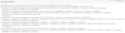
性別,年齢などが推定されている.
!cat test_outputs.csv
顔の性別,年齢等の予測を行う.
git clone https://github.com/dchen236/FairFace
公式の GitHub のページ: https://github.com/dchen236/FairFace
2つのファイルをダウンロードする.
「fair_face_models」という名前のディレクトリを作る. そして,いまダウンロードしたファイルのファイル名を次のように変えて, 「fair_face_models」ディレクトリの下に置く. (ファイル名については,predict.py の中で指定されているファイル名にあわせる)
cd FairFace
python predict.py --csv test_imgs.csv
test_imgs.csv には,次の画像ファイルのファイル名が設定されている.
自前の画像で動作確認したいときは,画像ファイル名を書いた csv ファイルを準備する
性別,年齢などが推定されている.
type test_outputs.csv
Fashion MNIST データセットは,10 種類のモノクロ画像と,各画像に付いた ラベル(10 種類の中の種類を示す)から構成されるデータセットである.
(内訳)70000枚の内訳は次の通りである
60000枚:教師データ
10000枚:検証データ
Fashion MNIST データセットは,次の URL で公開されているデータセット(オープンデータ)である.
URL: https://github.com/zalandoresearch/fashion-mnist
【関連情報】
【関連項目】 Keras に付属のデータセット, MNIST データセット, TensorFlow データセット, オープンデータ, 画像分類
次の Python プログラムは,TensorFlow データセットから,Fashion MNIST データセットのロードを行う. x_train, y_train が学習用のデータ.x_test, y_test が検証用のデータになる.
次の Python プログラムでは,TensorFlow データセットから,Fashion MNIST データセットのロードを行う. x_train と y_train を 25枚分表示することにより,x_train と y_train が,モノクロ画像であることが確認できる.
tensorflow_datasets の loadで, 「batch_size = -1」を指定して,一括読み込みを行っている.
from __future__ import absolute_import, division, print_function, unicode_literals
import tensorflow.compat.v2 as tf
tf.enable_v2_behavior()
print(tf.__version__)
import numpy as np
import tensorflow_datasets as tfds
%matplotlib inline
import matplotlib.pyplot as plt
import warnings
warnings.filterwarnings('ignore')   # Suppress Matplotlib warnings
%matplotlib inline
import matplotlib.pyplot as plt
import warnings
warnings.filterwarnings('ignore')   # Suppress Matplotlib warnings
# MNIST データセットのロード
mnist, mnist_metadata = tfds.load('mnist', with_info = True, shuffle_files=True, as_supervised=True, batch_size = -1)
x_train, y_train, x_test, y_test = mnist['train'][0], mnist['train'][1], mnist['test'][0], mnist['test'][1]
plt.style.use('default')
plt.figure(figsize=(10,10))
for i in range(25):
    plt.subplot(5,5,i+1)
    plt.xticks([])
    plt.yticks([])
    plt.grid(False)
# squeeze は,サイズ1の次元を削除.numpy は tf.Tensor を numpy に変換
    plt.imshow(np.squeeze(x_train[i]), cmap=plt.cm.binary)
    plt.xlabel(y_train[i].numpy())
# 確認表示
plt.show()
次の Python プログラムは,Keras に付属のデータセットの中にある Fashion MNIST データセットのロードを行う. x_train, y_train が学習用のデータ.x_test, y_test が検証用のデータになる.
from tensorflow.keras.datasets import fashion_mnist
(x_train, y_train), (x_test, y_test) = fashion_mnist.load_data()
次の Python プログラムは,Keras に付属のデータセットの中にある Fashion MNIST データセットのロードを行う. x_train と y_train を 25枚分表示することにより,x_train と y_train が,モノクロ画像であることが確認できる.
import tensorflow.keras
from tensorflow.keras.datasets import fashion_mnist
%matplotlib inline
import matplotlib.pyplot as plt
import warnings
warnings.filterwarnings('ignore')   # Suppress Matplotlib warnings
# Fashion MNIST データセットのロード
(x_train, y_train), (x_test, y_test) = fashion_mnist.load_data()
plt.style.use('default')
plt.figure(figsize=(10,10))
for i in range(25):
    plt.subplot(5,5,i+1)
    plt.xticks([])
    plt.yticks([])
    plt.grid(False)
    plt.imshow(x_train[i], cmap=plt.cm.binary)
    plt.xlabel(y_train[i])
# 確認表示
plt.show()
【TensorFlow データセット から Fashion MNIST データセット をロード】
結果は,TensorFlow の Tensor である.
type は型,shape はサイズ,np.max と np.mi は最大値と最小値.
tensorflow_datasets の loadで, 「batch_size = -1」を指定して,一括読み込みを行っている.
from __future__ import absolute_import, division, print_function, unicode_literals
import tensorflow.compat.v2 as tf
tf.enable_v2_behavior()
print(tf.__version__)
import numpy as np
import tensorflow_datasets as tfds
%matplotlib inline
import matplotlib.pyplot as plt
import warnings
warnings.filterwarnings('ignore')   # Suppress Matplotlib warnings
# Fashion MNIST データセットのロード
fashion_mnist, fashion_mnist_metadata = tfds.load('fashion_mnist', with_info = True, shuffle_files=True, as_supervised=True, batch_size = -1)
x_train, y_train, x_test, y_test = fashion_mnist['train'][0], fashion_mnist['train'][1], fashion_mnist['test'][0], fashion_mnist['test'][1]
print(fashion_mnist_metadata)
# 【x_train, x_test, y_train, y_test の numpy ndarray への変換と,値の範囲の調整(値の範囲が 0 〜 255 であるのを,0 〜 1 に調整)】
x_train = x_train.numpy().astype("float32") / 255.0
x_test = x_test.numpy().astype("float32") / 255.0
y_train = y_train.numpy()
y_test = y_test.numpy()
print(type(x_train), x_train.shape, np.max(x_train), np.min(x_train))
print(type(x_test), x_test.shape, np.max(x_test), np.min(x_test))
print(type(y_train), y_train.shape, np.max(y_train), np.min(y_train))
print(type(y_test), y_test.shape, np.max(y_test), np.min(y_test))
ICP の一手法
Fast-Robust-ICP のページ(Git Hub): https://github.com/yaoyx689/Fast-Robust-ICP
【関連項目】 K 近傍探索 (K nearest neighbour), ICP
次のコマンドやプログラムは Google Colaboratory で動く(コードセルを作り,実行する).
実行でのオプションについては,Fast-Robust-ICP のページ(Git Hub): https://github.com/yaoyx689/Fast-Robust-ICP
C++ ビルドツール (Build Tools) のインストール, cmake のインストール, Eigen 3 のインストール, Git のインストール が必要.
cd c:\
rmdir /s /q Fast-Robust-ICP
git clone --recursive https://github.com/yaoyx689/Fast-Robust-ICP
cd Fast-Robust-ICP
rmdir /s /q build
mkdir build
cd build
cmake -G "Visual Studio 16 2019" -T host=x64 ^
    -DCMAKE_BUILD_TYPE=Release ^
    -DCMAKE_INSTALL_PREFIX="c:/Fast-Robust-ICP" ^
    -DEIGEN3_INCLUDE_DIRS="c:/;c:/eigen" ^
..
cmake --build . --config RELEASE
cmake --build . --config RELEASE --target INSTALL
FERET データベースは顔のデータベース.詳細情報は,次のWebページにある.
https://www.nist.gov/itl/products-and-services/color-feret-database
【関連項目】 顔のデータベース
FFHQ (Flickr-Faces-HQ) データセット は,70,000枚の顔画像データセット. 機械学習による顔の生成などの学習や検証に利用できるデータセットである.
FFHQ (Flickr-Faces-HQ) データセットは次の URL で公開されているデータセット(オープンデータ)である.
URL: https://github.com/NVlabs/ffhq-dataset
【関連情報】
A Style-Based Generator Architecture for Generative Adversarial Networks, Tero Karras (NVIDIA), Samuli Laine (NVIDIA), Timo Aila (NVIDIA), CoRR, abs/1812.04948
【関連項目】 顔のデータベース
FFmpeg は,動画のデコーダとエンコーダに関するソフトウエア.
FFmpeg の公式ページ: https://ffmpeg.org/
学習済みモデルを使用する. 学習済みモデルの一部に新しいモデルを合わせた上で,追加のデータを使い学習を行う. このとき,学習済みモデルの部分と,新しいモデルの部分の両方について,パラメータ(重みなど)の調整を行う.
【関連項目】 画像分類 (image classification), 分類, 物体検出
woctezuma の Google Colaboratory のページを使用する
このプログラムは,物体検出等の機能を持つモデルである DETR を使い, fine tuning (ファイン・チューニング)と,物体検出を行う.
COCO データセットで学習済みの DETR について,確認のため, 物体検出を行ったあと, 風船(baloon)についてのfine tuning (ファイン・チューニング)を行い, 風船(baloon)が検出できるようにしている. 風船(baloon)は,COCO データセット には無い.
!pip3 uninstall -y torchtext
!pip3 install torch==1.8.0 torchvision==0.9.0 torchtext==0.9.0
import torch, torchvision
print(torch.__version__, torch.cuda.is_available())
torch.set_grad_enabled(False);
COCO データセットのクラス名を確認する.
orange, apple, banana, doc, person などがある.baloon は無い.
detr_resnet50 の事前学習済みのモデルをダウンロードしている.
しきい値 0.9, 0.7, 0.0 の 3 通りで実行.しきい値を下げるほど,検出できる物体は増えるが,誤検知も増える傾向にある.
fine tuning を行うため,風船 (baloon) の画像,そして,風船の領域を示した情報(輪郭線,包含矩形)の情報を使う. 画像は複数.そのうち1枚は次の通り.
過学習は起きていないようである
fine tuning により,風船(baloon)を検出できるようになった. しきい値は 0.9, 0.7 の 2通り.
そのフォーマットは,/content/data/custom (Google Colaboratory の data/custom の下のファイル)が参考になる.
自前のデータが準備できたら,Google Colaboratory にアップロードし, 次のコードセルの「/content/data/custom」のところを書き換えて,再度実行する.
最初の物体検知(fine tuning の前)で,別の画像で試したいとき.
画像ファイルをアップロード.プログラムは次のように書き換える.
fname = '/content/5m126sn2pov30qzu3pc49lampcp6.jpg'
im = Image.open(fname)
scores, boxes = detect(im, detr, transform)
URL: https://github.com/woctezuma/finetune-detr
flann は近似近傍探索の機能を持ったソフトウエア
flann のインストールは,複数の方法がある.
ここでは, vcpkg を使う方法を説明する.
c:\vcpkg\vcpkg search flann
c:\vcpkg\vcpkg install flann[hdf5] hdf5
c:\vcpkg\installed\x64-windows\bin
ディープラーニングにより姿勢推定を行うためのデータとして利用できる.
次の URL で公開されているデータセット(オープンデータ)である. http://bensapp.github.io/flic-dataset.html
【関連情報】
Sapp, B., Taskar, B.: Modec: Multimodal decomposable models for human pose estimation. In: Computer Vision and Pattern Recognition (CVPR), 2013 IEEE Conference on, IEEE (2013) 3674–3681, https://www.cv-foundation.org/openaccess/content_cvpr_2013/papers/Sapp_MODEC_Multimodal_Decomposable_2013_CVPR_paper.pdf
FordA データセットは,時系列データである.
FordA データセットは,公開されているデータセット(オープンデータ)である.
URL: http://www.timeseriesclassification.com/description.php?Dataset=FordA
教師データ数:3601
テストデータ数: 1320
モーターセンサーにより計測されたエンジンノイズの計測値.
20種類, 約 42.5 時間分のサウンドである.
次の URL で公開されているデータセット(オープンデータ)である.
http://www.eduardofonseca.net/FSDnoisy18k/
Eduardo Fonseca, Manoj Plakal, Daniel P. W. Ellis, Frederic Font, Xavier Favory, and Xavier Serra, “Learning Sound Event Classifiers from Web Audio with Noisy Labels”, arXiv preprint arXiv:1901.01189, 2019
【関連項目】 sound data
URL: https://www.iai.kit.edu/1302.php
Windows での FZKViewer のインストールは 別ページで説明している.
FZKViewer で CityGML のファイルを開くときは, File, Open, Open GML File... と操作する.
ファイルが読み込まれると,次のように表示される.
【関連項目】 CityGML
帰無仮説: 正規分布に従う2群の標準偏差が等しい . F 検定を,t 検定の行う前の等分散性の検定に使うのは正しくないという指摘もある.
R システム で,2群 s1, s2 の F 検定を行うプログラム
var.test(s1, s2)
【関連項目】 検定
GAN (Generative Adversarial Network) では, 生成器 (generator) でデータを生成し, 識別機 (discriminator) で,生成されたデータが正当か正当でないかを識別する.
Ian J. Goodfellow, Jean Pouget-Abadie, Mehdi Mirza, Bing Xu, David Warde-Farley, Sherjil Ozair, Aaron Courville, Yoshua Bengio, Generative Adversarial Networks, Proceedings of the 27th International Conference on Neural Information Processing Systems 2014
【関連項目】 Applications of Deep Neural Networks, Real-ESRGAN, TecoGAN, Wasserstein GAN (WGAN), Wasserstein GAN with Fradient Penalty (WGAN-GP) ディープラーニング
git はバージョン管理のソフトウエア.Windows 版の git の1つ「git for Windows」には,MinGWが同封されている.
git の URL: https://git-scm.com/
Windows での git のインストールには,複数の方法がある.次のいずれかによりインストールできる.
winget をインストールしたのち,コマンドプロンプトを管理者として実行し,「winget install Git」を実行
詳しくは 別ページで説明している.
Ubuntu での git のインストールは, 端末で,次のコマンドを実行.
sudo apt -y update
sudo apt -y install git
Google アカウントは,Google のオンラインサービス等の利用のときに使うアカウント. Google オンラインサービスの利用条件などは,利用者で確認すること.
Google アカウントの取得: 別ページで説明している.
Google Colaboratory の利用により, オンラインで,Web ブラウザを用いて,次のことができる.
Google Colaboratory は,オンラインで使用する. Google Colaboratory の使用には,Google アカウントの取得が必要.
詳しくは: 別ページで説明している.
Google Colaboratory のコードセルで,次の Python プログラムを実行
import tensorflow as tf
print(tf.__version__)
import keras
print(keras.__version__)
Google Colaboratory のコードセルで,次の Python プログラムを実行
!nvcc -V
Google Colaboratory のコードセルで,次の Python プログラムを実行
import torch
CUDA_VERSION = torch.__version__.split("+")[-1]
print(CUDA_VERSION)
!nvidia-smi --query-gpu=gpu_name,driver_version,memory.total --format=csv
try:
    from google.colab import drive
    USE_COLAB = True
except:
    USE_COLAB = False
Google Colaboratory での実行結果
Windows のコマンドプロンプトでの実行結果
GPU は,グラフィックス・プロセッシング・ユニットの略で、コンピュータグラフィックス関連の機能,乗算や加算の並列処理の機能などがある.
Graphviz はグラフデータ構造の機能を持ったソフトウエアである.
URL: https://graphviz.gitlab.io/
Windows での Graphviz のインストールには,複数の方法がある.次のいずれかによりインストールできる.
詳しくは 別ページで説明している.
インストールの終了後,C:\Program Files\Graphviz\bin にパスを通す.
Ubuntu での graphviz のインストール
sudo apt -y update
sudo apt -y install graphviz libgraphviz-dev python3-graphviz
grep は,正規表現で,テキストファイルの中から行を選択する機能を持つソフトウエア.
Windows での環境変数の設定は,マイコンピュータを右クリック → プロパティ→ 詳細設定 → 環境変数をクリック
Windowsの画面の表示では、「\」(円マーク)が表示される
He らの方法 (2015年) では,前層のユニット数(ニューロン数)を n とするとき, sqrt( 2 / n ) を標準偏差とする正規分布に初期化する. ただし,この方法は ReLU に特化した手法であるとされている. この方法を使うとき,層の入力は,正規化済みであること.
Kaiming He, Xiangyu hang, Shaoqing Ren and Jian Sun, Delving Deep into Rectifiers: Surpassing Human-Level, Performance on ImageNet Classification, pp. 1026^1-34.
HDF5 のインストールは,複数の方法がある.
ここでは, vcpkg を使う方法を説明する.
c:\vcpkg\vcpkg search hdf5
c:\vcpkg\vcpkg install hdf5[zlib] zlib
c:\vcpkg\installed\x64-windows\bin
HELENデータセットは,顔画像と,顔のパーツの輪郭のデータセットである.
次の URL で公開されているデータセット(オープンデータ)である.
http://www.ifp.illinois.edu/~vuongle2/helen/
【関連情報】
【関連項目】 顔のデータベース
HMDB51 (a large human motion database) データセット は,人間の行動データセット. 機械学習による行動分類,行動認識,ビデオ検索などの学習や検証に利用できるデータセットである.
HMDB51 (a large human motion database) データセット >は次の URL で公開されているデータセット(オープンデータ)である.
https://serre-lab.clps.brown.edu/resource/hmdb-a-large-human-motion-database/#introduction
【関連情報】
Hour Grass Network は,stacked hourglass と呼ばれるアーキテクチャを特色とする CNN (convolutional neural network) である.
姿勢推定 (pose estimation) は,画像から,関節 (joint) の (x,y) 座標を得たり, ヒートマップを得る(ヒートマップでは,画素ごとに値を持ち,その値は,関節である確率が高いほど,高い値になる) 姿勢制御では,さまざまなスケールでの情報を扱うことが課題とされ, stacked hourglass で解決できるとされている. hougrass では,最初にプーリングを行い,その後アップサンプリングを行う. hougrass を直接に並べて stacked hourglass を構成する.
Hour Grass Network の文献は次の通りである.
A. Newell, K. Yang, and J. Deng. Stacked hourglass net- works for human pose estimation. In ECCV, 2016, CoRR, abs/1603.06937.
https://arxiv.org/pdf/1603.06937v2.pdf
【関連項目】 姿勢推定
Hour Grass Network を用いた姿勢推定については,次の文献がある.
qhttps://github.com/bearpaw/pytorch-pose
上の文献では,ディープラーニングにより,人体全身の姿勢推定を行っている. その学習は,次の手順で行う
git clone https://github.com/bearpaw/pytorch-pose
py -3.6 -m pip install scipy==1.1.0 imutils easydict progress
py -3.6 -m pip install torch==1.9.0+cu111 torchvision==0.10.0+cu111 torchaudio===0.9.0 -f https://download.pytorch.org/whl/torch_stable.html
cd pytorch-pose
mkdir .\checkpoint
mkdir .\checkpoint\mpii
mkdir .\checkpoint\mpii\hg_s1_b1
# MPII データセットを用いた学習
py -3.6 .\example\main.py --dataset mpii --arch hg --stack 1 --block 1 --features 256 --checkpoint .\checkpoint\mpii\hg_s1_b1 --anno-path .\data\mpii\mpii_annotations.json --image-path .\mpii\images
ディープラーニングにより姿勢推定を行うためのデータとして利用できる.
利用には, https://vision.imar.ro/human3.6m/register.php での申請を必要とする.
http://vision.imar.ro/human3.6m/description.php
Catalin Ionescu, Dragos Papava, Vlad Olaru and Cristian Sminchisescu, Human3.6M: Large Scale Datasets and Predictive Methods for 3D Human Sensing in Natural Environments, IEEE Transactions on Pattern Analysis and Machine Intelligence, vol. 36, No. 7, July 2014
iBUG 300-W データセットは, 顔の 68 ランドマーク のデータである.7764枚の顔画像について,手作業で,顔の 68 ランドマークのアノテーションとラベル付が行われている.
顔ランドマーク (facial landmark)は,目,眉,鼻,口,あごのラインなど,顔のパーツの構造を特定でぃる形状予測器 (shape predictor) の学習に使うことができる.
iBUG 300-W データセットの URL: https://ibug.doc.ic.ac.uk/resources/300-W/
【関連項目】 顔の 68 ランドマーク, 顔ランドマーク (facial landmark), 顔のデータベース
画像の中で,除去する対象となるオブジェクトの境界などを指定することにより, 指定されたオブジェクトを除去し,除去された部分の画素は, image completion and extrapolation で補う.
次の文献では, 除去する対象となるオブジェクトの境界を正確に指定しなくても, オブジェクトスコアマップ (object score map) を scene parsing network を用いて 推定することにより, image content removal(画像コンテンツの除去)ができるとされている.
この論文の手法の SunkskyF による実装は,次のページで公開されている.
https://github.com/SunskyF/StructCompletion-python
実行の前準備として,「pip install -U opencv-python opencv-contrib-python」を実行する.demo.py の実行結果は次のとおりである.
【関連項目】 image completion and extrapolation
「100x」のように x を付ける.
convert -resize 100x -unsharp -quality 100 fruits.jpg 1.jpg
「100x」のように x を付ける.
こちらは,元ファイルを上書き
mogrify -resize 100x -unsharp -quality 100 fruits.jpg
for i in *.png; do
if [ `identify -format "%[width]" $i` -gt 440 ]; then
    echo $i
    mogrify -resize 440x -unsharp 0x1+0.5+0 -quality 100 $i
fi
done
【関連項目】 画像データの形式変換
Windows でのインストールは,別ページで説明している.
Ubuntu でインストールを行うには,端末で,次のコマンドを実行する.
sudo apt -y update
sudo apt -y install imagemagick
前景の色を F,背景の色を B とし,元画像の色は I = alpha * F + (1 - alpha) * B とする. 元画像 I は既知であり,F, B, alpha は未知であるとする. このとき alpha を推定することを image matting という(alpha image matting ともいう).
写真や動画の前景背景分離に用いることができる. 物体検出 や salient object detection との違いとしては, ガラスなどの半透明なもの,髪の毛や網のようなもの,そして,前景が必ずしも画面中央に集まっているとは限らず,画面全域にある(網越しに外を見るような場合)を想定していることがある.
【関連情報】
【関連項目】 AIM-500 (Automatic Image Matting-500) データセット
trimap では,次の 3つを考える. 前景である画素は白,背景である画素は黒,transaction である画素は灰色の 3通りに 塗り分けた画像を trimap という.
Trimap-based matting では, 元画像と,その trimap を用いて image matting を行う. ディープラーニングによる Trimap-based matting の手法としては,Xu らの Deep Image Matting (DIM) (2017年)(文献 [1]) などが知られている.
【関連情報】
Ning Xu, Brian Price, Scott Cohen, Thomas Huang, Deep Image Matting CVPR 2017, CoRR, https://arxiv.org/abs/1703.03872v3
Backgroud matting は,image matting において背景画像を用いる. つまり,元画像と,追加の背景画像を用いて image matting を行う. 元画像での背景と,追加の背景画像は同一の場所で撮影されたものが想定されている.そのとき,全に一致しなくてもよい(わずかな位置のずれや照明条件の変化は許容される).
ディープラーニングによるbackground matting Shanchuan Lin らの Backgroud Matting (2021年)(文献 [2])などが知られる. Backbone に ResNet-50, ASPP (Atrous Spatial Pyramid Pooling, DeepLabV3 のものに従う).
Background matting では,Trimap を必要としない. ZOOM などのビデオ会議などで,グリーンバックを使わずに,前景と背景を分離するとき, 背景の取得は容易であり, Background matting は有用である.
【関連情報】
Shanchuan Lin, Andrey Ryabtsev, Soumyadip Sengupta, Brian Curless, Steve Seitz, Ira Kemelmacher-Shlizerman, Real-Time High-Resolution Background Matting CVPR 2021, also CoRR, https://arxiv.org/abs/2012.07810v1, 2021.
https://arxiv.org/pdf/2012.07810v1.pdf
人物や動物に特化した image matting である. 人物や動物が写った写真や動画に対して,image matting を行う. このとき,Trimap や 背景画像などの追加の情報を準備することなく image matting を行う手法が種々提案されている.
Trimap や 背景画像などの追加の情報を必要とせず, 人物や動物など以外でも(例えば,半透明のコップ,網ごしの風景写真など) image matting を行うもの. Li らの GFM (文献 [3])(2020 年)は,ディープラーニングによる Trimap の推定が行われており, Li らの unified semantic model (文献 [4])(2021 年)は,Salient Opaque, Salient Transparent/Meticulous, Non-Salient の 3種類の画像を扱えるモデルであり,GGM の拡張により,unified semantic model の推定を行っている.
Jizhizi Li, Jing Zhang, Stephen J Maybank, and Dacheng Tao. End-to-end animal image matting. arXiv preprint arXiv:2010.16188, 2020.
Jizhizi Li , Jing Zhang and Dacheng Tao, Deep Automatic Natural Image Matting, 2021. https://arxiv.org/pdf/2107.07235v1.pdf
ImageNet データセット は,画像分類や物体検出 のベンチマークである「ImageNet Large Scale Visual Recognition Challenge(ILSVRC)」で使用されている. 機械学習での画像分類 や物体検出 の学習や検証に利用できるデータセットである.
ImageNet データセットは次の URL で公開されているデータセット(オープンデータ)である.
ImageNet データセットの URL: https://image-net.org/
【関連情報】
IMDb の URL: https://www.imdb.com/
IMDb での映画の批評は,批評文とスコア(10点満点)である. IMDb データセットでは,7点以上の批評は positive,4点以下の批評は negative としている.つまり,2種類ある. そして,IMDb データセットには,positive か negative の批評のみが含まれている(中間の点数である 5点,6点のものは含まれていない).そして, positive,negative の批評が同数である. 学習用として,positive,negative がそれぞれ 25000. 検証用として,positive,negative がそれぞれ 25000.
IMDb データセットのURL: https://ai.stanford.edu/%7Eamaas/data/sentiment/
【関連項目】 Keras に付属のデータセット, TensorFlow データセット, オープンデータ,
次の Python プログラムは,TensorFlow データセットから,IMDb データセットのロードを行う. x_train, y_train が学習用のデータ.x_test, y_test が検証用のデータになる.
次のプログラムでは,そして確認表示を行う.
tensorflow_datasets の loadで, 「batch_size = -1」を指定して,一括読み込みを行っている.
from __future__ import absolute_import, division, print_function, unicode_literals
import tensorflow.compat.v2 as tf
tf.enable_v2_behavior()
print(tf.__version__)
import numpy as np
import tensorflow_datasets as tfds
%matplotlib inline
import matplotlib.pyplot as plt
import warnings
warnings.filterwarnings('ignore')   # Suppress Matplotlib warnings
imdb_reviews, imdb_reviews_metadata = tfds.load('imdb_reviews', with_info = True, shuffle_files=True, as_supervised=True, batch_size = -1)
x_train, y_train, x_test, y_test = imdb_reviews['train'][0], imdb_reviews['train'][1], imdb_reviews['test'][0], imdb_reviews['test'][1]
# 確認表示
import pandas as pd
display(pd.DataFrame(x_train[0:14], y_train[0:14]))
IMDb データセットは,次のプログラムでロードできる.
【Keras のプログラム】
from tensorflow.keras.datasets import imdb
(x_train, y_train), (x_test, y_test) = imdb.load_data()
40種類の人間の顔を撮影した240枚の画像. 58個の顔ランドマークが付いている.
URL: http://www2.imm.dtu.dk/pubdb/pubs/3160-full.html
M. M. Nordstr{\o}m and M. Larsen and J. Sierakowski and M. B. Stegmann, The IMM Face Database - An Annotated Dataset of 240 Face Images
http://www2.imm.dtu.dk/pubdb/edoc/imm3160.pdf
【関連項目】 顔のデータベース
画像のデータセット.アノテーションとしてバウンディングボックスが付けられている.Imbalance の大きさを特徴とする.
次の URL で公開されているデータセット(オープンデータ)である.
URL: https://github.com/visipedia/inat_comp/tree/master/2017
顔検出 (face detection),顔のアラインメント, 顔検証 (face verification), 顔識別 (face identification)の機能を持つ.
InsightFace の GitHub のページ: https://github.com/deepinsight/insightface
【関連項目】 ArcFace 法, Chandrika Deb の顔マスク検出, Dlib の顔検出, face alignment, MobileFaceNets, 顔検出 (face detection)
公式ページ (https://github.com/deepinsight/insightface/tree/master/python-package) に記載の顔検出及び年齢と性別の予測のプログラムを変更して実行.
このプログラムは buffalo_l という名前の事前学習済みモデルを使用している.
次のコマンドやプログラムは Google Colaboratory で動く(コードセルを作り,実行する).
GPU を使わない場合には「onnxruntime-gpu」でなく,「onnxruntime」をインストールすること.
!pip3 install -U insightface onnxruntime-gpu opencv-python numpy
動作確認のため,公式ページ (https://github.com/deepinsight/insightface/tree/master/python-package) に記載の,顔検出及び年齢と性別の予測のプログラムを実行する.
このプログラムは buffalo_l という名前の事前学習済みモデルを使用している.
このプログラムの実行により,result.jpg ファイルができる.
import cv2
import numpy as np
%matplotlib inline
import matplotlib.pyplot as plt
import insightface
from insightface.app import FaceAnalysis
from insightface.data import get_image as ins_get_image
app = FaceAnalysis(providers=['CUDAExecutionProvider', 'CPUExecutionProvider'])
app.prepare(ctx_id=0, det_size=(640, 640))
img = ins_get_image('t1')
faces = app.get(img)
rimg = app.draw_on(img, faces)
plt.style.use('default')
plt.imshow(cv2.cvtColor(rimg, cv2.COLOR_BGR2RGB))
plt.show()
cv2.imwrite("./result.jpg", rimg)
顔の画像ファイルは何でも良いが,ここでは,画像ファイルをダウンロードしている.
!curl -O https://www.kkaneko.jp/sample/face/3284.png
!curl -O https://www.kkaneko.jp/sample/face/3285.png
!curl -O https://www.kkaneko.jp/sample/face/3287.png
!curl -O https://www.kkaneko.jp/sample/face/3288.png
!curl -O https://www.kkaneko.jp/sample/face/3289.png
!curl -O https://www.kkaneko.jp/sample/face/3290.png
いま準備した画像ファイルについて,顔検出及び年齢と性別の予測の実行
import cv2
import numpy as np
%matplotlib inline
import matplotlib.pyplot as plt
import insightface
from insightface.app import FaceAnalysis
from insightface.data import get_image as ins_get_image
app = FaceAnalysis(providers=['CUDAExecutionProvider', 'CPUExecutionProvider'])
app.prepare(ctx_id=0, det_size=(640, 640))
img = cv2.imread('3284.png')
faces = app.get(img)
rimg = app.draw_on(img, faces)
plt.style.use('default')
plt.imshow(cv2.cvtColor(rimg, cv2.COLOR_BGR2RGB))
plt.show()
img = cv2.imread('3285.png')
faces = app.get(img)
rimg = app.draw_on(img, faces)
plt.style.use('default')
plt.imshow(cv2.cvtColor(rimg, cv2.COLOR_BGR2RGB))
plt.show()
img = cv2.imread('3287.png')
faces = app.get(img)
rimg = app.draw_on(img, faces)
plt.style.use('default')
plt.imshow(cv2.cvtColor(rimg, cv2.COLOR_BGR2RGB))
plt.show()
img = cv2.imread('3288.png')
faces = app.get(img)
rimg = app.draw_on(img, faces)
plt.style.use('default')
plt.imshow(cv2.cvtColor(rimg, cv2.COLOR_BGR2RGB))
plt.show()
img = cv2.imread('3289.png')
faces = app.get(img)
rimg = app.draw_on(img, faces)
plt.style.use('default')
plt.imshow(cv2.cvtColor(rimg, cv2.COLOR_BGR2RGB))
plt.show()
img = cv2.imread('3290.png')
faces = app.get(img)
rimg = app.draw_on(img, faces)
plt.style.use('default')
plt.imshow(cv2.cvtColor(rimg, cv2.COLOR_BGR2RGB))
plt.show()
Google Colaboratory では, Python, PyTorch はインストール済みなので,インストール操作は不要.
コマンドプロンプトを管理者として実行し,次のコマンドを実行.
GPU を使わない場合には「onnxruntime-gpu」でなく,「onnxruntime」をインストールすること.
python -m pip install -U insightface onnxruntime-gpu opencv-python numpy
動作確認のため,公式ページ (https://github.com/deepinsight/insightface/tree/master/python-package) に記載の,顔検出及び年齢と性別の予測のプログラムを実行する.
このプログラムは buffalo_l という名前の事前学習済みモデルを使用している.
このプログラムの実行により,result.jpg ファイルができる.
import cv2
import numpy as np
import insightface
from insightface.app import FaceAnalysis
from insightface.data import get_image as ins_get_image
app = FaceAnalysis(providers=['CUDAExecutionProvider', 'CPUExecutionProvider'])
app.prepare(ctx_id=0, det_size=(640, 640))
img = ins_get_image('t1')
faces = app.get(img)
rimg = app.draw_on(img, faces)
plt.style.use('default')
plt.imshow(cv2.cvtColor(rimg, cv2.COLOR_BGR2RGB))
plt.show()
cv2.imwrite("./result.jpg", rimg)
import cv2
import numpy as np
import insightface
from insightface.app import FaceAnalysis
from insightface.data import get_image as ins_get_image
app = FaceAnalysis()
app.prepare(ctx_id=0, det_size=(640, 640))
v = cv2.VideoCapture(0)
while(v.isOpened()):
    r, f = v.read()
    if ( r == False ):
        break
    faces = app.get(f)
    rimg = app.draw_on(f, faces)
    cv2.imshow("", rimg)
    if cv2.waitKey(1) & 0xFF == ord('q'):
        break
![[image]](../db/30.png)
前準備として,Python のインストール, PyTorch のインストール を行う.
Google Colaboratory では, Python, PyTorch はインストール済みなので,インストール操作は不要.
次に,pip を用いて,pillow のインストールを行う.
pip install -U pillow
Ubuntu でインストールを行うには,端末で,次のコマンドを実行する.
GPU を使わない場合には「onnxruntime-gpu」でなく,「onnxruntime」をインストールすること.
sudo apt -y update
sudo apt -y install python3-numpy libopencv-dev libopencv-core-dev python3-opencv libopencv-contrib-dev opencv-data
sudo pip3 install -U insightface onnxruntime-gpu
動作確認のため,公式ページ (https://github.com/deepinsight/insightface/tree/master/python-package) に記載の,顔検出及び年齢と性別の予測のプログラムを実行する.
このプログラムは buffalo_l という名前の事前学習済みモデルを使用している.
このプログラムの実行により,result.jpg ファイルができる.
import cv2
import numpy as np
import insightface
from insightface.app import FaceAnalysis
from insightface.data import get_image as ins_get_image
app = FaceAnalysis(providers=['CUDAExecutionProvider', 'CPUExecutionProvider'])
app.prepare(ctx_id=0, det_size=(640, 640))
img = ins_get_image('t1')
faces = app.get(img)
rimg = app.draw_on(img, faces)
plt.style.use('default')
plt.imshow(cv2.cvtColor(rimg, cv2.COLOR_BGR2RGB))
plt.show()
cv2.imwrite("./result.jpg", rimg)
import cv2
import numpy as np
import insightface
from insightface.app import FaceAnalysis
from insightface.data import get_image as ins_get_image
app = FaceAnalysis()
app.prepare(ctx_id=0, det_size=(640, 640))
v = cv2.VideoCapture(0)
while(v.isOpened()):
    r, f = v.read()
    if ( r == False ):
        break
    faces = app.get(f)
    rimg = app.draw_on(f, faces)
    cv2.imshow("", rimg)
    if cv2.waitKey(1) & 0xFF == ord('q'):
        break
Iris データセットは公開されているデータセット(オープンデータ)である.
Iris データセットについての説明資料を準備している: iris.pdf [PDF], [パワーポイント]
次の Python プログラムは,Iris データセットのロードと確認表示を行う. Pandas データフレームの df にロードしている. 確認表示で display を用いている.
import pandas as pd
from sklearn.datasets import load_iris
from IPython.display import display
iris = load_iris()
df = pd.DataFrame(iris.data, columns=iris.feature_names)
df['species'] = iris.target_names[iris.target]
display(df)
次の Python プログラムは,Iris データセットのロードと確認表示を行う.配列 X, y にロードしている. 確認表示で display を用いている.
import pandas as pd
from sklearn.datasets import load_iris
from IPython.display import display
iris = load_iris()
x = iris.data
y = iris.target
display(x)
display(y)
URL: https://github.com/google/jax
Ubuntu でインストールを行うには,端末で,次のコマンドを実行する.
sudo apt -y install python3-pip
sudo pip3 install -U "jax[cuda111]" -f https://storage.googleapis.com/jax-releases/jax_releases.html
国別,地域別の感染者データ
URL: https://github.com/CSSEGISandData/COVID-19
次の Python プログラムは, Johns Hopkins 大の COVID-19 データレポジトリからデータをダウンロードし,ロードし,表示する.
!curl -LO https://github.com/CSSEGISandData/COVID-19/raw/master/csse_covid_19_data/csse_covid_19_time_series/time_series_covid19_confirmed_global.csv
import pandas as pd
df = pd.read_csv("./time_series_covid19_confirmed_global.csv")
display(df)
display(df.groupby(['Country/Region'], as_index=False).sum())
【関連項目】 時系列データ
Jupyter Lab は Python プログラム作成に関する種々の機能を持ったソフトウエア.
JupyterLab について:別ページ で説明している.
Jupyter Qt Console は Python コンソールの機能を持ったソフトウエア.
Jupyter Qt Console について:別ページ で説明している.
Jupyter ノートブックは,Pythonなどのプログラムのソースコード,実行結果などを1つのノートとして残す機能をもったノートブック.
Jupyter ノートブック について:別ページ で説明している.
Keras は 機械学習のAPI の機能を持つ. Python 言語から利用可能. TensorFlow, CNTK, Theano など,さまざまなディープラーニングのフレームワークの上で動く.
参考 Web ページ
Keras の概要
次のプログラムでは,損失関数を, categorical crossentropy, 最適化法を 確率的勾配降下法 (SGD 法), 尺度を accuracy に設定している.
m.compile(optimizer=tf.keras.optimizers.SGD(lr=0.01, momentum=0.9, nesterov=True),
          loss='sparse_categorical_crossentropy',
          metrics=['accuracy'])
※ 目的関数については: https://keras.io/ja/objectives/
【関連項目】 Applications of Deep Neural Networks, TensorFlow, ディープラーニング
Avatar Erik Linder-Norén により GitHub で公開されているKeras-GAN のページ.
URL は次の通り.
Keras-GAN のページ: https://github.com/eriklindernoren/Keras-GAN
次のプログラムの中の kernel_initializer の部分. 標準偏差を 0.01 になるように重みを設定している.
【Keras のプログラム】
m.add(Dense(units=100, input_dim=len(768[0])), kernel.iniializer.TruncatedNormal(stddev=0.01))
教師データ x_train と y_train (x_train は入力データの numpy 配列もしくは numpy 配列のリスト,y_train はクラス番号の numpy 配列)を用いて, バッチサイズが 32,エポック数を 10 として学習したいときには,次のコマンドを用いる.
【Keras のプログラム】
history = m.fit(x_train, y_train, batch_size=32, epochs=50, validation_data=(x_test, y_test))
Keras での学習において,「validation_data」を付けることで,検証(バリデーション)が行われる.
このとき,検証(バリデーション)に使うデータ(x_test, y_test)をいろいろ変えながら,Kerasでの検証(バリデーション)を行う.
【Keras のプログラム】
history = m.fit(x_train, y_train, batch_size=32, epochs=50, validation_data=(x_test, y_test))
結果(上のプログラムでは history)を見て,過学習や学習不足を判断する.history は次のようなプログラムで表示できる.
【Keras のプログラム】
import pandas as pd
h = pd.DataFrame(history.history)
h['epoch'] = history.epoch
print(h)
Keras のモデルのコンパイルにおいては, オプティマイザ(最適化器)と 損失関数とメトリクスの指定を行う必要がある.
Keras でのモデル m のコンパイルのプログラムは「m.compile」のように書く.
データセットは,データの集まりのこと. Python の keras には,次のデータセットを簡単にダウンロードできる機能がある.
CIFAR-10 データセットは,次のプログラムでロードできる.
【Keras のプログラム】
from tensorflow.keras.datasets import cifar10
(x_train, y_train), (x_test, y_test) = cifar10.load_data()
CIFAR-100 データセットは,次のプログラムでロードできる.
【Keras のプログラム】
from tensorflow.keras.datasets import cifar100
(x_train, y_train), (x_test, y_test) = cifar100.load_data(label_mode='fine')
IMDb データセットは,次のプログラムでロードできる.
【Keras のプログラム】
from tensorflow.keras.datasets import imdb
(x_train, y_train), (x_test, y_test) = imdb.load_data()
Reuters newswire topics データセットは,次のプログラムでロードできる.
【Keras のプログラム】
from tensorflow.keras.datasets import reuters
(x_train, y_train), (x_test, y_test) = reuters.load_data()
MNIST データセットは,次のプログラムでロードできる.
【Keras のプログラム】
from tensorflow.keras.datasets import mnist
(x_train, y_train), (x_test, y_test) = mnist.load_data()
Fashion MNIST データセットは,次のプログラムでロードできる.
【Keras のプログラム】
from tensorflow.keras.datasets import fashion_mnist
(x_train, y_train), (x_test, y_test) = fashion_mnist.load_data()
Boston housing price 回帰データセットは,次のプログラムでロードできる.
【Keras のプログラム】
from tensorflow.keras.datasets import boston_housing
(x_train, y_train), (x_test, y_test) = boston_housing.load_data()
keras に付属のデータセットを取得するときのオプションについては, https://keras.io/ja/datasets/(日本語版), https://keras.io/datasets/(英語版) に説明されている.
【関連項目】 Boston housing price 回帰データセット, CIFAR-10 データセット, CIFAR100 データセット, IMDb データセット, Reuters newswire topics データセット, MNIST データセット, Fashion MNIST データセット
Keras の応用としては, MobileNetV2, Inception-ResNet, ResNet50, DenseNet121, DenseNet169, NASNetなどの画像分類のモデルがある. (その詳細は,https://keras.io/ja/applications/)
Keras では,これらモデルについて,ImageNet データセット での学習済みモデルを,次のようなプログラムで,簡単に使えるようにすることができる.
【Keras のプログラム】
from tensorflow.keras.applications.mobilenet_v3 import MobileNetV3
m = MobileNetV3(weights='imagenet')
【関連項目】 ResNet50, ResNet101, ResNet152, その他の ResNet, Inception-ResNet, DenseNet121, DenseNet169, NASNet, MobileNetV2
Keras で利用可能な画像分類のモデルは,https://keras.io/api/applications/ で説明されている.
400/600/700 種類の人間の行動をカバーする最大65万のビデオクリップの URL リンク集とアノテーションである. それぞれのクリップには,1つの行動クラスがアノテーションされている. ビデオの長さは,約10秒である. 機械学習による行動分類,行動認識,ビデオ検索などの学習や検証に利用できるデータセットである.
ディープラーニングで,人間の行動推定に利用できる.
Kinetics データセット >は次の URL で公開されているデータセット(オープンデータ)である.
https://deepmind.com/research/open-source/kinetics
【関連情報】
W. Kay, J. Carreira, K. Simonyan, B. Zhang, C. Hillier, S. Vijayanarasimhan, F. Viola, T. Green, T. Back, P. Natsev, M. Suleyman, and A. Zisserman. The kinetics human action video dataset. arXiv preprint arXiv:1705.06950, 2017.
次のコマンドは Google Colaboratory で動く(コードセルを作り,実行する).
!curl -O https://storage.googleapis.com/deepmind-media/Datasets/kinetics700_2020.tar.gz
!tar -xvzof kinetics700_2020.tar.gz
!ls kinetics700_2020
mkdir c:\data
mkdir c:\data\kinetics
cd c:\data\kinetics
curl -O https://storage.googleapis.com/deepmind-media/Datasets/kinetics700_2020.tar.gz
"c:\Program Files\7-Zip\7z.exe" x kinetics700_2020.tar.gz
"c:\Program Files\7-Zip\7z.exe" x kinetics700_2020.tar
カラーのカメラ,モノクロのステレオカメラ,3次元レーザースキャナなどのさまざまなセンサーのデータから構成される.
http://www.cvlibs.net/datasets/kitti
【関連情報】
【関連項目】 semantic segmentation, オープンデータ, 物体検出
https://github.com/navoshta/KITTI-Dataset
https://github.com/utiasSTARS/pykitti
K 近傍探索 (K nearest neighbour)のアルゴリズムは,次の性質を持つ.
【関連項目】 Fast-Robust-ICP, libnabo, libpointmatcher
ks_1033_data は,次のページで CSV ファイルと Excel ファイルで公開されているデータセット(オープンデータ)である.
https://github.com/wireservice/csvkit/tree/master/examples/realdata
次のコマンドは Google Colaboratory で動く(コードセルを作り,実行する).
!curl -O https://github.com/wireservice/csvkit/tree/master/examples/realdata/ks_1033_data.csv
!ls -al ks_1033_data.csv
正則化の一手法である. L2 正則化では,重みの二乗の合計に比例したペナルティを,重みに与える.
L2 正則化を行う Keras のプログラム
L2 正則化を行いたいときは 次のようにする.
import tensorflow.compat.v2 as tf
tf.keras.layers.Dense(128, activation='relu', kernel_regularizer=tf.keras.regularizers.l2(0.001))
LabelMe インタフェースは,アノテーションのツール.
Russell BC, Torralba A, Murphy KP, Freeman WT, Labelme: a database and web-based tool for image annotation. Int’l Journal of Computer Vision, 2008.
【関連項目】 アノテーション (annotation)
公式ページ https://github.com/wkentaro/labelmeの記載に従う.
LaMa は,Image Inpainting (イメージインペインティング)のための技術である.2021年発表.
Image Inpainting (イメージインペインティング) 画像の欠落部分を補うことで,画像の中の不要な部分を消すときにも役立つ.
LaMa のデモページ
![[image]](../db/164.png)
【関連項目】 image inpainting
lapack は,行列に関する種々の問題(連立1次方程式,固有値問題,などなど多数)を解く機能を持つソフトウエア.BLAS の機能を使う.
netlib の lapack のページ: http://www.netlib.org/lapack
lapack 参照実装の Web ページ: https://github.com/Reference-LAPACK/lapack-release
LAPACK のインストールは,複数の方法がある.
ここでは, vcpkg を使う方法を説明する.
c:\vcpkg\vcpkg search lapack
c:\vcpkg\vcpkg install blas lapack lapack-reference openblas[threads]:x64-windows
c:\vcpkg\installed\x64-windows\bin
Ubuntu でインストールを行うには,端末で,次のコマンドを実行する.
sudo apt -y update
sudo apt -y install libopenblas-dev liblapack-dev
スポーツ選手を中心としで,Flickr から収集した2000枚の画像に, 姿勢(ポース)についてのアノテーションを行ったもの. 最も目立つ人物が,およそ150ピクセルになるようにスケーリングされている. 各画像には,14個のジョイント(関節)の位置がアノテーションされている. オリジナル画像の帰属 (attribution) とFlickrのURLは,各画像ファイルのJPEGコメントに記載されている.
ディープラーニングにより姿勢推定を行うためのデータとして利用できる.
次の URL で公開されているデータセット(オープンデータ)である.
URL: http://sam.johnson.io/research/lsp.html
Sam Johnson, and Mark Everingham. Clustered Pose and Nonlinear Appearance Models for Human Pose Estimation. In Frédéric Labrosse, Reyer Zwiggelaar, Yonghuai Liu, and Bernie Tiddeman, editors, Proceedings of the British Machine Vision Conference, pages 12.1-12.11. BMVA Press, September 2010. doi:10.5244/C.24.12.
http://www.bmva.org/bmvc/2010/conference/paper12/paper12.pdf
https://github.com/open-mmlab/mmpose/blob/master/docs/en/tasks/3d_body_mesh.md#lsp
次のコマンドは Google Colaboratory で動く(コードセルを作り,実行する).
アノテーションファイルは,次の URL からダウンロードできる.
https://drive.google.com/open?id=1GZxlTLuMfA3VRvz2jyv8fhJDqElNrgKS
Windows の場合.次により c:\data\lsp にダウンロードされる.
アノテーションファイルは,次の URL からダウンロードできる.
https://drive.google.com/open?id=1GZxlTLuMfA3VRvz2jyv8fhJDqElNrgKS
Ubuntu の場合.次により,/usr/local/data/lsp/images にダウンロードされる.
アノテーションファイルは,次の URL からダウンロードできる.
https://drive.google.com/open?id=1GZxlTLuMfA3VRvz2jyv8fhJDqElNrgKS
LFWデータセットには,「in-the-wild」のラベル付きの顔のデータベースである.
合計で 13,233枚,5,749人の顔画像が含まれている.
機械学習による顔認識の学習や検証に利用できるデータセットである.
Gary B. Huang, Marwan Mattar, Tamara Berg, Eric Learned-Miller. Labeled Faces in the Wild:
A Database for Studying Face Recognition in Unconstrained Environments. Workshop on Faces in
’Real-Life’ Images: Detection, Alignment, and Recognition, Erik Learned-Miller and Andras Ferencz
and Frdric Jurie, Oct 2008, Marseille, France. inria-00321923
【関連項目】
顔認識 (face recognition),
顔のデータベース
libiconv のインストールは,複数の方法がある.
ここでは,
vcpkg を使う方法を説明する.
libnabo は,K 近傍探索 (K nearest neighbour) の機能を持つライブラリ.
ANN よりも高速だとされている.
Elseberg, J. and Magnenat, S. and Siegwart, R. and N{\"u}chter, A.,
Comparison of nearest-neighbor-search strategies and implementations for efficient shape registration,
Journal of Software Engineering for Robotics (JOSER), pages 2-12, vol. 3, no. 1, 2012.
【関連項目】
K 近傍探索 (K nearest neighbour)
https://github.com/CAOR-MINES-ParisTech/libpointmatcher/blob/master/doc/CompilationWindows.md の手順に従う.
Boost のインストール,
C++ ビルドツール (Build Tools) のインストール,
Eigen 3 のインストール,
Git のインストール,
grep のインストール
が必要.
Visual Studio の x64 Native Tools コマンドプロンプトを管理者として実行する.
次のコマンドを実行する.
c:\libnabo にインストールされる.
Visual Studio の x64 Native Tools コマンドプロンプトを管理者として実行する.
次のコマンドを実行する.
c:\libnabo にインストールされる.
Ubuntu でインストールを行うには,端末で,次のコマンドを実行する.
/usr/local/libnabo にインストールされる.
Iterative Closest Point (ICP) の機能を持ち,
点群 (point cloud) のアラインメントを行うことができる.
point-to-point の ICP と,point-to-plane ICP の機能を持つ.
point-to-point の ICP では,剛体変換だけでなく,スケールの変更にも対応している.
François Pomerleau, Francis Colas, Roland Siegwart, Stéphane Magnenat,
Comparing ICP Variants on Real-World Data Sets,
Autonomous Robots, vol. 34, no. 3, pages: 133-148, 2013.
François Pomerleau, Stéphane Magnenat, Francis Colas, Ming Liu, Roland Siegwart,
Tracking a Depth Camera: Parameter Exploration for Fast ICP,
Proc. of the IEEE/RSJ International Conference on Intelligent Robots and Systems (IROS),
IEEE Press, pages: 3824-3829, 2011.
【関連項目】
K 近傍探索 (K nearest neighbour),
ICP
https://github.com/CAOR-MINES-ParisTech/libpointmatcher/blob/master/doc/CompilationWindows.md の手順に従う.
Boost のインストール,
C++ ビルドツール (Build Tools) のインストール,
cmake のインストール,
Eigen 3 のインストール,
Git のインストール,
libnabo のインストール,
が必要.
Visual Studio の x64 Native Tools コマンドプロンプトを管理者として実行する.
次のコマンドを実行する.
c:\libpointmatcher にインストールされる.
公式ページの
https://github.com/CAOR-MINES-ParisTech/libpointmatcher/blob/master/doc/CompilationWindows.md
libnabo のインストール が必要.
Ubuntu でインストールを行うには,端末で,次のコマンドを実行する.
/usr/local/libpointmatcher にインストールされる.
librosa は,
音声,音楽の機能をもった Python のパッケージである.
McFee, Brian, Colin Raffel, Dawen Liang, Daniel PW Ellis, Matt McVicar, Eric Battenberg, and Oriol Nieto. “librosa: Audio and music signal analysis in python.” In Proceedings of the 14th python in science conference, pp. 18-25. 2015.
【関連項目】
short-time Fourier transform,
音声, 音楽, sound,
音データ(sound data)
次のプログラムは Google Colaboratory で動く(コードセルを作り,実行する).
次のプログラムは,librosa に付属の音声データである trumpet について,パワースペクトログラムを表示する.
次のプログラムでは,横軸は時間,縦軸は線形スケール(linear scale)で表された周波数である
パワースペクトログラムを表示する.
stft は short-time Fourier transform を行う.
そして,その振幅により色をプロットする.
ここのプログラムのソースコードは,
http://librosa.org/doc/main/auto_examples/plot_display.html#sphx-glr-auto-examples-plot-display-py
のものを使用(ISC ライセンス).
Windows での librosa のインストールは,次のようなコマンドで行う.
コマンドプロンプトを管理者として実行し,次のコマンドを実行.
Ubuntu での librosa のインストールは,次のようなコマンドで行う.
インストールするバージョンを指定する場合には,次のように操作する.
「==」のあとはバージョン指定であり,使用したいバージョンを指定する.
ソースコードを使用してインストールする場合には次のように操作する.
Windows での LLVM のインストールには,複数の方法がある.次のいずれかによりインストールできる.
12.0.1 のところは,インストールしたいバージョン番号を指定すること.
Ubuntu でインストールを行うには,端末で,次のコマンドを実行する.
Linux では,locate コマンドを用いてファイル検索を行うことができる.
画像の類似尺度.Richard Zhang らにより 2018年に提案された.
公式ページには,次の Python プログラムのソースコードが掲載されている.
このソースコードの Google Colaboratory での実行結果は次の通りである.
Richard Zhang, Phillip Isola, Alexei A. Efros, Eli Shechtman, Oliver Wang,
The Unreasonable Effectiveness of Deep Features as a Perceptual Metric,
CVPR 2018, also CORR, abs/1801.03924v2
【関連項目】SSIM
LReLU (Leaky rectified linear unit) は,次の関数である.
f(x) = x (x>=0), alpha * x (x<0)
LReLUは,活性化関数としてよく使用されるもののうちの1つである.
活性化関数は,ニューロンの入力の合計から,そのニューロンの活性度の値を決めるためのもの.
(他には,ReLU,シグモイド関数,ステップ関数,ソフトマックス関数などがある.
LS3D-W データセットは,3次元の顔ランドマーク (facial landmark)のデータセット.
これは,AFLW,300VW,iBUG 300-W,FDDB の顔画像から生成されたデータセットである.
利用には,
https://www.adrianbulat.com/face-alignment
での申請を必要とする.
生成手順については,次の文献に記載されている
Bulat, Adrian and Tzimiropoulos, Georgios,
International Conference on Computer Vision,
2017,
https://openaccess.thecvf.com/content_ICCV_2017/papers/Bulat_How_Far_Are_ICCV_2017_paper.pdf
【関連項目】
顔ランドマーク (facial landmark)
LSTM 層を含むようなニューラルネットワークは,次の特徴を持つ
【関連項目】
Applications of Deep Neural Networks,
ディープラーニング,
リカレントニューラルネットワーク
LSTM 層では,内部に「状態」を維持する.
状態は,ニューロンの動作のたびに変化するものである.
(ふつうのニューロンでは,入力の値から出力が計算される.「状態」という考え方はない).
LSTM 層のニューロンは,今の入力,1つ前の時間の入力,1つ前の時間での状態から出力を求める.
LSUN (Large-scale Scene UNderstanding Challenge) データセット は,
ラベル付きの画像データセットである.
機械学習での画像分類や画像生成の学習や検証に利用できるデータセット.
LSUN データセットは次の URL で公開されているデータセット(オープンデータ)である.
【関連情報】
Fisher Yu, Ari Seff, Yinda Zhang, Shuran Song, Thomas Funkhouser and Jianxiong Xiao,
LSUN: Construction of a Large-scale Image Dataset using Deep Learning with Humans in the Loop,
arXiv:1506.03365
【関連項目】 顔のデータベース
機械学習による物体検出では,
「mAP」は,「mean average precision」の意味である.
ストリート(街角)の25,000 枚の画像.
インスタンスレベルのアノテーション,
124 のセマンティッククラス.
次の URL で公開されているデータセット(オープンデータ)である.
URL: https://www.mapillary.com/dataset/vistas
G. Neuhold, T. Ollmann, S. Rota Bulo, and P. Kontschieder.
The mapillary vistas dataset for semantic understanding of
street scenes. In ICCV, 2017.
【関連項目】
semantic segmentation, インスタンス・セグメンテーション (instance segmentation)
セグメンテーション,物体検出,キーポイント検出等に使用されるモデル.
FPN (Feature Pyramid Network), ResNeXt101 や ResNeXt50 や ResNet101 や ResNet50 を使用.
COCO データセットで学習済みのモデル,Jupyter ノートブック (Jupyter Notebook) のデモ demo.ipynb が公開されている.
【関連項目】
PANet (Path Aggregation Network),
物体検出,
segmentation,
keypoint detection
Jupyter ノートブック (Jupyter Notebook) のデモが付属している.主なものは次の通り.
動作させるには,Mask R-CNN のインストールが終わっていること(下に記載).
学習: train_shapes.ipynb
仕組み: inspect_model.ipynb
重みの視覚化: inspect_weights.ipynb
matplotlib は,オープンソースの Python のプロットライブラリ.
matplotlib を用いた散布図の描画は,別ページで説明している.
matplotlib を用いたグラフ描画の例は次の通り.
matplotlib を用いて,OpenCV のカラー画像を表示する例は次の通り.
普通に Matplotlib を用いてOpenCV 画像の表示を表示すると,小さく表示される.
「plt.style.use('default')」の実行により,Matplotlib での OpenCV 画像の表示が大きくなる.
【サイト内の関連ページ等】
Matplotlib(Python まとめページ内)
【関連項目】
display
Windows での matplotlib, seaborn のインストールは,
コマンドプロンプトを管理者として実行し,
そのコマンドプロンプトで,次のコマンドを実行することで行う.
Ubuntu での matplotlib, seaborn のインストールは,
次のコマンドを実行することで行う.
画像からの物体検出 のための学習法である.
当時の,従来の,単純な物体検出 法よりも高速であり,
他の種々の物体検出 法よりも精度が劣らないとされている.
サブサンプリングを行わずに,サブウインドウ(画像分類のために使用されるもの)の全体での最適化を行うことを特徴としている.
Davis E. King, Max-Margin Object Detection, CoRR, abs/1502.00046, 2015.
【関連項目】 物体検出
MeCab は,形態素解析の機能を持ったソフトウエア.
Windows での MeCab のインストールには,複数の方法がある.次のいずれかによりインストールできる.
ここでは,
vcpkg を使う方法を説明する.
MeshLab は, 3次元データ(3次元点群データや,メッシュデータ)について表示, 簡易編集, データの間引き, 形式変換, 張り合わせ, 分割, 解析などが行えるソフトウエア
URL: http://meshlab.sourceforge.net/
【関連項目】
メッシュ簡略化 (Mesh Simplification) ,
メッシュ平滑化 (Mesh Smoothing)
Windows での MeshLab のインストールには,複数の方法がある.次のいずれかによりインストールできる.
詳しくは: 別ページで説明している.
Meshroom は Structure from Motion を,GUI を用いて簡単に行えるソフトウエア.動作画面の一部は次の通り.カメラの撮影位置と,オブジェクトの3次元形状が表示されている.
meshroom の URL (ここから Meshroom をダウンロード可能): https://alicevision.org/
【関連項目】
3次元再構成 (3D reconstruction),
OpenMVG,
OpenMMLab,
Structure from Motion (SfM)
ADE20K データセット から派生した,
シーン解析(scene parsing) のデータと,
オブジェクトのパーツ (object parts) のセグメンテーションのデータ.
次の URL で公開されているデータセット(オープンデータ)である.
http://sceneparsing.csail.mit.edu/
【関連情報】
【関連項目】
ADE20K データセット,
CASILVision,
semantic segmentation,
シーン解析(scene parsing),
インスタンス・セグメンテーション (instance segmentation)
c:\date 下にダウンロード,展開する.
コマンドプロンプトを管理者として実行し,次のコマンドを実行.
ファイルの配置は次のようになる.
キャラクタと動きのアセットを公開しているサイト.fbx形式でダウンロードできる.
【関連用語】
3次元コンピュータグラフィックス, human pose, human motion
MMClassification は,
OpenMMLab の構成物で,
画像分類のツールボックスとベンチマークの機能を提供する.
MMCV Contributors, MMCV: OpenMMLab Computer Vision Foundation,
https://github.com/open-mmlab/mmcv, 2018.
【関連項目】
OpenMMLab
次のコマンドやプログラムは Google Colaboratory で動く(コードセルを作り,実行する).
https://mmclassification.readthedocs.io/en/latest/install.html の記載の手順による
MMClassificationの公式の事前学習済みモデルの説明: https://github.com/open-mmlab/mmclassification/tree/master/configs/resnet
「demo/demo.JPEG」のところに画像ファイル名を指定する.
「demo/demo.JPEG」のところに画像ファイル名を指定する.
「demo/demo.JPEG」のところに画像ファイル名を指定する.
「demo/demo.JPEG」のところに画像ファイル名を指定する.
MMCV は,
OpenMMLab の構成物で,基礎的な機能を提供する.
MMCV Contributors, MMCV: OpenMMLab Computer Vision Foundation,
https://github.com/open-mmlab/mmcv, 2018.
【関連項目】
OpenMMLab
次のコマンドやプログラムは Google Colaboratory で動く(コードセルを作り,実行する).
https://mmcv.readthedocs.io/en/latest/get_started/installation.html に記載の手順による
NVIDIA CUDA ツールキット 11.1, PyTorch 1.10 がインストール済みの場合には,次のようになる
「cu111/torch1.10」のところは,
NVIDIA CUDA ツールキット のバージョン,
PyTorch のバージョンに合わせる.
バージョンについては,公式のページ https://github.com/open-mmlab/mmcv に説明がある.
インストールの方法は複数ある.
ここでは,
NVIDIA CUDA ツールキットを使うことも考え,
インストールしやすい方法として,ソースコードからビルドしてインストールする方法を案内している.
Ubuntu でインストールを行うには,端末で,次のコマンドを実行する.
MMDetection は,
OpenMMLab の構成物で,物体検出の機能を提供する.
Chen, Kai and Wang, Jiaqi and Pang, Jiangmiao and Cao, Yuhang and
Xiong, Yu and Li, Xiaoxiao and Sun, Shuyang and Feng, Wansen and
Liu, Ziwei and Xu, Jiarui and Zhang, Zheng and Cheng, Dazhi and
Zhu, Chenchen and Cheng, Tianheng and Zhao, Qijie and Li, Buyu and
Lu, Xin and Zhu, Rui and Wu, Yue and Dai, Jifeng and Wang, Jingdong
and Shi, Jianping and Ouyang, Wanli and Loy, Chen Change and Lin, Dahua,
MMDetection: Open MMLab Detection Toolbox and Benchmark,
arXiv:1906.07155, 2019.
次のコマンドやプログラムは Google Colaboratory で動く(コードセルを作り,実行する).
https://github.com/open-mmlab/mmdetection/blob/master/docs/en/get_started.md に記載の手順による
あとで使用する
インストールの方法は複数ある.
ここでは,
NVIDIA CUDA ツールキットを使うことも考え,
インストールしやすい方法として,ソースコードからビルドしてインストールする方法を案内している.
「git checkout v2.14.0」は,バージョン 2.14.0 を指定している.
これは,https://mmdetection3d.readthedocs.io/en/latest/getting_started.html#installation での2021/08 時点の説明による.将来はバージョン番号が変わる可能性があり,このページを確認してから,インストールを行うこと.
カレントディレクトリをc:\mmdetection にして実行すること.
「git checkout v2.14.0」は,バージョン 2.14.0 を指定している.
これは,https://mmdetection3d.readthedocs.io/en/latest/getting_started.html#installation での2021/08 時点の説明による.将来はバージョン番号が変わる可能性があり,このページを確認してから,インストールを行うこと.
Ubuntu でインストールを行うには,端末で,次のコマンドを実行する.
Ubuntu の場合は,
mmcv のドキュメント: https://mmcv.readthedocs.io/en/latest/
の手順がそのまま使えそうである.
MMSegmentation は,
OpenMMLab の構成物で,物体検出の機能を提供する.
MMSegmentation Contributors,
MMSegmentation: OpenMMLab Semantic Segmentation Toolbox and Benchmark,
https://github.com/open-mmlab/mmsegmentation, 2020.
次のコマンドやプログラムは Google Colaboratory で動く(コードセルを作り,実行する).
https://mmcv.readthedocs.io/en/latest/get_started/installation.html に記載の手順による
NVIDIA CUDA ツールキット 11.1, PyTorch 1.10 がインストール済みの場合には,次のようになる
「cu111/torch1.10」のところは,
NVIDIA CUDA ツールキット のバージョン,
PyTorch のバージョンに合わせる.
バージョンについては,公式のページ https://github.com/open-mmlab/mmcv に説明がある.
インストールの方法は複数ある.
ここでは,
NVIDIA CUDA ツールキットを使うことも考え,
インストールしやすい方法として,ソースコードからビルドしてインストールする方法を案内している.
「git checkout v0.14.1」は,バージョン 0.14.1 を指定している.
これは,https://mmdetection3d.readthedocs.io/en/latest/getting_started.html#installation での2021/08 時点の説明による.将来はバージョン番号が変わる可能性があり,このページを確認してから,インストールを行うこと.
CityScapes データセットを用いての事前学習済みモデルを使用している.
カレントディレクトリをc:\segmentation にして実行すること.
エラーメッセージが出ないことを確認.
「git checkout v0.14.1」は,バージョン 0.14.1 を指定している.
これは,https://mmdetection3d.readthedocs.io/en/latest/getting_started.html#installation での2021/08 時点の説明による.将来はバージョン番号が変わる可能性があり,このページを確認してから,インストールを行うこと.
Ubuntu でインストールを行うには,端末で,次のコマンドを実行する.
Ubuntu の場合は,
MMCV のドキュメント: https://mmsegmentation.readthedocs.io/en/latest/get_started.html#verification
の手順がそのまま使えそうである.
Google Colaboratory でのインストールは,次のような手順になるようである(未確認).
MMSelfSup は,
OpenMMLab の構成物で,
Self-Supervised Representation Learning の機能を提供する.
MMSelfSup Contributors,
MMSelfSup: OpenMMLab Self-Supervised Learning Toolbox and Benchmark,
https://github.com/open-mmlab/mmselfsup, 2021.
【関連項目】
MMCV,
MMDetection,
MMSegmentation,
OpenMMLab,
Self-Supervised Representation Learning,
物体検出
次のコマンドやプログラムは Google Colaboratory で動く(コードセルを作り,実行する).
MMSelfSup のインストール(公式ページ): https://github.com/open-mmlab/mmselfsup/blob/master/docs/en/install.md
https://github.com/open-mmlab/mmdetection/blob/master/docs/en/get_started.md に記載の手順による
公式ページ
https://github.com/open-mmlab/mmselfsup/blob/master/docs/en/install.md
に記載のプログラムを実行してみる.
エラーメッセージが出なければ OK.
MMTracking は,
OpenMMLab の構成物で,トラッキングビジョンの機能を提供する.
次のコマンドやプログラムは Google Colaboratory で動く(コードセルを作り,実行する).
https://github.com/open-mmlab/mmdetection/blob/master/docs/en/get_started.md に記載の手順による
あとで使用する
mot.mp4 というファイルができるので,ダウンロードして表示
0 から 9 までの 10 種類の手書き文字についての,
モノクロ画像と,各画像に付いた「0から9までの数値」のラベルから構成されるデータセットである.
(内訳)70000枚の内訳は次の通りである
60000枚:教師データ
10000枚:検証データ
MNIST データセットは,公開されているデータセット(オープンデータ)である.
【関連情報】
【関連項目】
Keras に付属のデータセット,
Fashion MNIST データセット,
TensorFlow データセット,
オープンデータ,
画像分類
次の Python プログラムは,TensorFlow データセットから,MNIST データセットのロードを行う.
x_train, y_train が学習用のデータ.x_test, y_test が検証用のデータになる.
次のプログラムでは,x_train と y_train を 25枚分表示することにより,x_train と y_train が,手書き文字のモノクロ画像であることが確認できる.
tensorflow_datasets の loadで,
「batch_size = -1」を指定して,一括読み込みを行っている.
【TensorFlow データセット から MNIST データセット をロード】
結果は,TensorFlow の Tensor である.
type は型,shape はサイズ,np.max と np.mi は最大値と最小値.
tensorflow_datasets の loadで,
「batch_size = -1」を指定して,一括読み込みを行っている.
次の Python プログラムは,Keras に付属のデータセットの中にある MNIST データセットのロードを行う.
x_train, y_train が学習用のデータ.x_test, y_test が検証用のデータになる.
次のプログラムは、MNIST データセットのロードを行う.x_train と y_train を 25枚分表示することにより,x_train と y_train が,手書き文字のモノクロ画像であることが確認できる.
顔検証 (face verification) を,その当時の従来の mobile networks よりも高速で高精度で実行できるとされている.
InsightFace などで実装されている.
Sheng Chen, Yang Liu, Xiang Gao, Zhen Han,
MobileFaceNets: Efficient CNNs for Accurate Real-Time Face Verification on Mobile Devices,
CCBR 2018, also CoRR, abs/1804.07573v, 2018.
https://arxiv.org/ftp/arxiv/papers/1804/1804.07573.pdf
【関連項目】
InsightFace,
顔検証 (face verification),
顔に関する処理
MobileNet は,separable convolution を特徴としている.ResNet の高速化が達成できたとされている.
MobileNetV2 は,conv 1x1, depthsise conv, conv 1x1 を特徴としている.高速化が達成できたとされている.
MobileNetV2 は、ディープラーニングでの画像分類などの高速化、精度向上のため
Depthwise Separable Convolution という考え方が導入されていることが特徴である.
Keras の MobileNetV2 を用いて MobileNetV2 を作成するプログラムは次のようになる.
「weights=None」を指定することにより,最初,重みをランダムに設定する.
【Keras のプログラム】
Keras の応用のページ: https://keras.io/ja/applications/
【サイト内の関連ページ】
Andrew Howard, Mark Sandler, Grace Chu, Liang-Chieh Chen, Bo Chen, Mingxing Tan, Weijun Wang, Yukun Zhu, Ruoming Pang, Vijay Vasudevan, Quoc V. Le, Hartwig Adam,
Searching for MobileNetV3, ICCV 2019
関連項目: 画像分類
Google Colab あるいはパソコン(Windows あるいは Linux)を使用.
前準備として,Python のインストール,
PyTorch のインストール を行う.
Google Colaboratory では,
Python, PyTorch はインストール済みなので,インストール操作は不要.
次に,pip を用いて,pillow のインストールを行う.
PyTorch, torchvision のモデルについては: https://pytorch.org/vision/stable/models.html に説明がある.
「m.eval()」は,推論を行うときのためのもの.これを行わないと訓練(学習)が行われる.
Google Colaboratory での結果
Windows での結果
Linux での結果
MPII Human Pose データセット は,
人体全身の画像と姿勢のデータセットである.
ディープラーニングにより姿勢推定を行うためのデータとして利用できる.
40,000人以上の人間を含む約25,000枚の画像が含まれている.
(28,000 が訓練データ,11,000 が検証データである).
画像のアノテーションが行われている.
410 種類の人間の活動を網羅している.
各画像については,活動名のラベルが付いている.
画像はYouTubeの動画から抽出されたものである.
テストデータセットでは,体のオクルージョン,胴体や頭の3次元での向きなど,
より豊富なアノテーションが行われている.
次の URL で公開されているデータセット(オープンデータ)である.
URL: http://human-pose.mpi-inf.mpg.de/
ライセンス: BSD ライセンス.利用条件等は,利用者で確認すること.
【関連情報】
https://openaccess.thecvf.com/content_cvpr_2014/papers/Andriluka_2D_Human_Pose_2014_CVPR_paper.pdf
Mykhaylo Andriluka and Leonid Pishchulin and Peter Gehler and Schiele, Bernt,
2D Human Pose Estimation: New Benchmark and State of the Art Analysis,
IEEE Conference on Computer Vision and Pattern Recognition (CVPR), 2014,
https://openaccess.thecvf.com/content_cvpr_2014/papers/Andriluka_2D_Human_Pose_2014_CVPR_paper.pdf
MS-Celeb-1M データセット を洗浄 (clean) したデータ.
画像サイズは 112x112.
RetinaFace を用いて推定された,5点の顔ランドマーク (facial landmark)が付いている.
人物数は 94,682 (94,682 identities), 画像数は 6,464,018 枚 (6,464,018 images)
次の URL で公開されているデータセット(オープンデータ)である.
https://github.com/EB-Dodo/C-MS-Celeb
【関連項目】
InsightFace,
MS-Celeb-1M データセット,
RetinaFace,
顔のデータベース,
顔ランドマーク (facial landmark),
顔検出 (face detection)
MS-Celeb-1M は,顔のデータセット.
このデータセットは,公開が撤回されている.
人物数は約 100,000 (100K identities), 画像数は約 8,000,000 枚 (8M images)
Yandong Guo, Lei Zhang, Yuxiao Hu, Xiaodong He, and Jianfeng Gao,
MS-Celeb-1M: A Dataset and Benchmark for Large-Scale Face Recognition,
In ECCV, 2016.
arXiv:1607.08221
【関連項目】
C-MS-Celeb Cleaned データセット ,
InsightFace,
顔のデータベース,
顔検出 (face detection)
MUCT 顔データベースは,3755名の顔のデータベース.手作業で 76個の顔ランドマーク (facial landmark)が付けらている.
MUCT 顔データベースは次の URL で公開されているデータセット(オープンデータ)である.
URL: https://www.cs.columbia.edu/CAVE/software/curet/html/about.php
URL: http://www.milbo.org/muct/index.html
S. Milborrow and J. Morkel and F. Nicolls,
The MUCT Landmarked Face Database,
Pattern Recognition Association of South Africa, 2010.
【関連項目】 顔のデータベース, 顔ランドマーク (facial landmark)
顔の 68 ランドマーク は,顔ランドマーク (facial landmark)の一種であり,68 組の数値で構成されている.68 組のそれぞれは,(x, y) 座標値である.
R. Gross, I. Matthews, J. Cohn, T. Kanade, and S. Baker,
Multi-pie, Image and Vision Computing, 28(5):807–813, 2010.
【関連項目】 顔の 68 ランドマーク の検出, 顔ランドマーク (facial landmark)
Multi View Stereo は,オブジェクトの低密度の3次元点群と,オブジェクトを周囲から撮影した多数の画像から,高密度の3次元点群を生成する.
【関連用語】
3次元再構成 (3D reconstruction),
meshroom,
OpenMVS,
Structure from Motion
Keras の NASNet を用いて NASNet を作成するプログラムは次のようになる.
「weights=None」を指定することにより,最初,重みをランダムに設定する.
【Keras のプログラム】
CoRR, abs/1707.07012
Keras の応用のページ: https://keras.io/ja/applications/
参考文献: http://www.cs.toronto.edu/~fritz/absps/momentum.pdf
NumPy は,オープンソースの Python のライブラリ.数値計算,行列の機能を持つ.
配列では,添え字が複数になる.
下に,Python の numpy 配列のコンストラクタの例を示す.
numpy 配列の形は shape 属性である.
numpy 配列の次元は ndim 属性である.
Windows での numpy のインストールは,
コマンドプロンプトを管理者として実行し,
次のコマンドを実行.
Ubuntu での numpy のインストールは,
次のコマンドで行う.
Nteractは,Pythonなどのプログラムのソースコード,実行結果などを1つのノートとして残す機能をもったノートブック.
NVIDIA CUDA ツールキット は,NVIDIA社が提供している GPU 用のプラットフォームである.
GPU は,グラフィックス・プロセッシング・ユニットの略で、コンピュータグラフィックス関連の機能,乗算や加算の並列処理の機能などがある.
NVIDIA 社のグラフィックスボードが持つ GPU の機能を使うとき,NVIDIA CUDA ツールキット を利用することができる.
NVIDIA CUDA ツールキットのインストールは,公式ページからインストール用のプログラムをダウンロードして実行.
NVIDIA cuDNN は,公式ページから ZIP ファイルをダウンロード,展開(解凍)し,パスを通す.
【サイト内の関連ページ】
関連 Web ページ
Ubuntu でのインストールは,次のページで説明している.
NVIDIA CUDA ツールキット のバージョンは何でも良いと言う場合には,apt を用いて,次の操作でインストールすることができる.
Ubuntu 20.04 バージョン 10.1 がインストールされる.
NVIDIA CUDA ツールキット,NVIDIA cuDNN については,次で情報を得ることができる.
次の公式ページを活用できる
Windows の場合は,コマンドプロンプトを管理者として実行し,次のコマンドを実行.
Ubuntu のシステム Python を使う場合は,次のコマンドを実行
Objectron は,3次元姿勢推定 (3D pose estimation) の機能を持つ.
Objectron は,次の公式ページで,プログラムとデータセットが配布されている.
https://github.com/google-research-datasets/Objectron
次は,Objectron の動作画面.
Objectron は,Google Colaboratory で動かすことができる.
Google Colaboratory で動かすときは,コードセルに,次の3行を張り付けて実行.
あとは,公式ページのプログラムのコピー&ペーストで動く.
【関連項目】
3次元姿勢推定 (3D pose estimation)
Objects365 データセットは,アノテーション済みの画像である.
機械学習での物体検出 の学習や検証に利用できるデータセット.
Objects365 データセットは次の URL で公開されているデータセット(オープンデータ)である.
https://www.objects365.org/overview.html
【関連情報】
one-hot エンコーディング (one-hot encodinng は,クラス番号を,長さがクラス数であるような数値ベクトルで,うち,1つだけが 1,残りが全て 0 になっているようなベクトルで表すこと.
1-of-k representation ともいう.
クラス番号が 0, 1, 2, 3 の 4通りであるとき,one hot 表現では [1 0 0 0] [0 1 0 0] [0 0 1 0] [0 0 0 1] のように表す.
Keras では,クラス番号を one hot 表現に変換するとき to_categorical 関数を用いる.
次の Python プログラムは,Iris データセットのロードを行う.配列 X, y にロードしている.
その後,訓練用データと検証用データへの分割と,one-hot エンコーディングを行っている.
確認表示で display を用いている.
帰無仮説: パラメトリック検定.等分散である多群の検定.平均に差がない.
R システム で,
one-way ANOVA (One-way analysis of variance) を行うプログラム.
one-way (一元配置) と言っているように,
x は必ず 1 つの数値である.
y は 1つの数値(カテゴリカル変数など)である.
【関連項目】
検定
ONNX のインストールは,複数の方法がある.
ここでは,
vcpkg を使う方法を使う方法を説明する.
Open3D は,3次元データに関する種々の機能を Python, C から扱うことができるソフトウエア.3次元再構成,サーフェスのアラインメント,可視化,PBR,3次元データに関する機械学習の機能を持つ.
インストール手順
まず,Python 3.6 あるいは 3.7 あるいは 3.8 をインストール.
次に,コマンドプロン
プトを管理者として実行する.
次のコマンドを実行
Open 3D Engine は,オープンソースの3次元ゲームエンジン.Amazon の Amazon Lumberyard の後継である.
o3de の URL: https://github.com/o3de/o3de
Windows での Open 3D Engine のインストール: 別ページで説明している.
BLAS(Basic Linear Algebra Subprograms)は,行列演算,ベクトル演算の機能をもったプログラム群である.
OpenBLAS の Web ページ: https://www.openblas.net/
【関連項目】 LAPACK
OpenBLAS のインストールは,複数の方法がある.
ここでは,
vcpkg を使う方法を説明する.
Ubuntu でインストールを行うには,端末で,次のコマンドを実行する.
OpenCV は,実時間コンピュータビジョン (real time computer vision) の アルゴリズムと文書とサンプルコードの集まり.
GitHub の OpenCV のページ: https://github.com/opencv/opencv/releases
【サイト内の関連資料や関連ページ】
【関連項目】 OpenCV のサンプルデータ
OpenCV のインストールは,複数の方法がある.
ここでは,
vcpkg を使う方法と,
公開されているパッケージを使う方法を説明する.
こちらの方法は,OpenCV の Python インタフェースのインストール法が私には分からなかったので,
Python インタフェースが不要な場合向けです.
こちらの方法は,OpenCV の Python インタフェースのインストール法が私には分からなかったので,
Python インタフェースが不要な場合向けです.
コマンドプロンプトを管理者として実行し,次のコマンドを実行.
バージョン 4.5.3 をインストールするときは,次の手順になる.他のバージョンをインストールするときは,「4.5.3」の部分をバージョン番号に読み替えること.
公式のインストール手順:
https://docs.opencv.org/4.5.5/d7/d9f/tutorial_linux_install.html
の通りに行う.
Ubuntu でインストールを行うには,端末で,次のコマンドを実行する.
OpenCV のサンプルデータ (samples/data) は,インターネットで公開されているデータセット(オープンデータ)である.(他のオープンデータと同様に,利用条件は利用者で確認すること).
curl を用いて,次のような操作でダウンロードできる.
不具合を避けるため,headless 版をインストールしている.
OpenGV は
Absolute camera pose computation,
Relative camera-pose computation,
Two methods for point-triangulation,
Arun's method for aligning point clouds
の機能を持つ.
Matlab, Python のインタフェースを持つ.
URL: https://laurentkneip.github.io/opengv/
論文:
L. Kneip, P. Furgale, “OpenGV: A unified and generalized approach to real-time calibrated geometric vision”, Proc. of The IEEE International Conference on Robotics and Automation (ICRA), Hong Kong, China. May 2014.
Ubuntu でインストールを行うには,端末で,次のコマンドを実行する.
OpenMMLab の URL: https://openmmlab.com/
OpenMMLab の GitHub のページ: https://github.com/open-mmlab
関連項目:
MMClassification,
MMCV,
MMDetection,
MMSegmentation,
MMSegmentation3D
MMTracking
OpenMVG は Structure from Motion の機能を持つソフトウエアソフトウエア.
OpenMVG が持っている Structure from Motion (SfM) の機能に,
Global Structure from Motion がある.
Global Structure from Motion は,
多数の視点からの画像を使う SfM において,視点の位置と向きの推定を(当時の手法よりも)より頑健かつ正確に推定できるとされている.
(その論文:
P. Moulon, P. Monasse and R. Marlet, "Global Fusion of Relative Motions for Robust, Accurate and Scalable Structure from Motion," 2013 IEEE International Conference on Computer Vision, 2013, pp. 3248-3255, doi: 10.1109/ICCV.2013.403.
https://www.researchgate.net/publication/261622957_Global_Fusion_of_Relative_Motions_for_Robust_Accurate_and_Scalable_Structure_from_Motion)
Windows での OpenMVG のインストールは,複数の方法がある.
ここでは,
vcpkg を使う方法と,
ソースコードからビルドする方法を説明する.
事前に Git のインストール,
cmake のインストール ,
Graphviz のインストールが必要.
コマンドプロンプトを管理者として実行し,次のコマンドを実行.
c:\openmvg にインストールされる.
OpenMVG (2021/08/21 時点) Windows 10 64 ビット版の非公式ビルド: openMVG.zip
私がビルドしたもの,非公式,無保証,ソースコードを改変せずにビルドした.OpenMVG の MPL2 ライセンスによる.
Ubuntu でインストールを行うには,端末で,次のコマンドを実行する.
デモプログラムとして,
所定の画像データセットをダウンロードし,SfM を実行する Python プログラムが付属している.
Windows では次の手順で行う.
デモプログラムの実行でできるファイルのうち,ply 形式ファイルの1つを MeshLabを用いて表示すると次のようになる.色付きの3次元点群である.
いくつかのコマンドを順に実行する.
Windows では次のような手順で行う.
最後の処理でできた,色付きの3次元点群のファイル(ply 形式ファイル)を MeshLabを用いて表示すると次のようになる.
続けて,次を実行する.上の結果を,OpenMVS を用いて処理している.実行には OpenMVS のインストールが必要
参考ページ: https://openmvg.readthedocs.io/en/latest/software/MVS/OpenMVS/ (公式の資料)
デモプログラムの実行でできるファイルのうち,ply 形式ファイルの1つを MeshLabを用いて表示すると次のようになる.色付きの3次元点群である.
OpenMVS は,Multi View Stereo の機能を持ったソフトウエア
【関連項目】
meshroom,
Multi View Stereo,
OpenMVG,
OpenMVS,
Structure from Motion (SfM)
Windows での OpenMVS のインストールは,複数の方法がある.
ここでは,
vcpkg を使う方法を説明する.
TensorFlow 2 で訓練ループのプログラムを書くときに利用できるソフトウエア.
Orbit の GitHub のページ:
https://github.com/tensorflow/models/tree/master/orbit
関連項目: TensorFlow
Panda3D は,オープンソースのソフトウエア,3次元ゲームエンジン (3-D game engine),可視化,シミュレーションの機能を持つ.
Panda3D の URL: https://www.panda3d.org/
TensorFlow などの機械学習フレームワークでは,入力として pandas のデータ構造をサポートしていることが多い.
【関連項目】
Iris データセット
次のようなプログラムでは,displayを用いて,Pandas のデータフレームを整形して表示している.
次の Python プログラムは,Iris データセットのロードと確認表示を行う.
Pandas データフレームの df にロードしている.
確認表示で display を用いている.
次の Python プログラムでは,次のことを行っている.
次の Python プログラムでは,to_numpy() を用いて,
Pandas データフレームを numpy.ndarray へ変換している.
Pandas のある特定の列(カラム)のデータについて,処理を繰り返したいときの書き方.iris は Iris データセットである.
Pandas のある特定の列(カラム)のデータについて,処理を繰り返すとき,ある条件(例えば 7 より大)のものだけ処理対象にしたいときの書き方
物体検出とインスタンス・セグメンテーション (instance segmentation)のためのネットワーク.
Mask R-CNN をもとに改善を行っている.
PANet のネットワークは,FPN バックボーンののち,
Bottom-up Path Augmentation を行い,
Adaptive Feature Pooling を行っている.
COCO データセット, CityScapes データセット, MVD データセットでの実験から,物体検出とインスタンス・セグメンテーション (instance segmentation)の精度が向上したとされている.
CSPNet の公式の実装 (GitHub) のページでは,
PANetを用いた物体検出として,
CSPDarknet53-PANet-SPP,
CSPResNet50-PANet-SPP,
CSPResNeXt50-PANet-SPP
等の実装が公開されている.
Shu Liu, Lu Qi, Haifang Qin, Jianping Shi, Jiaya Jia,
Path Aggregation Network for Instance Segmentation,
CVPR 2018, also CoRR, https://arxiv.org/abs/1803.01534v4,
【関連項目】
Mask R-CNN
物体検出, インスタンス・セグメンテーション (instance segmentation), YOLOv5
PARE は,3次元人体姿勢推定(3D human pose estimation)の技術である.
オクルージョンの問題を解決するために,
Part Attention REgressor (PARE) が提案されている.
multi person tracker を用いて実装されており,画像の中に複数の人物がいても動くようになっている.
PARE のデモプログラムの実行結果を次に示す.
この実行結果を得るためのもととなる動画: kaneko_sample_video.mp4
実行結果の動画: kaneko_sample_video__result.mp4
Kocabas, Muhammed and Huang, Chun-Hao P. and Hilliges, Otmar and Black, Michael J.,
PARE: Part Attention Regressor for {3D} Human Body Estimation,
Proc. International Conference on Computer Vision (ICCV),
also CoRR, abs/2104.08527v2, 2021.
【関連項目】
3D pose estimation,
3D human pose estimation,
YOLOv3,
multi person tracker
次のコマンドやプログラムは Google Colaboratory で動く(コードセルを作り,実行する).
前準備:事前に Python のインストール,
NVIDIA CUDA ツールキット,NVIDIA cuDNN のインストールを行うこと.
出来た動画を表示すると,次のように表示される.
PASCAL VOC データセットは,アノテーション済みの画像データ.
機械学習での物体検出 ,画像分類,セマンテック・セグメンテーションに利用できるデータセットである.
PASCAL VOC 2007, PASCAL VOC 2012 などいくつかの種類がある.
PASCAL VOC 2012 データセットの処す愛は次の通り.
vehicles, household, animals, and other: aeroplane, bicycle, boat, bus, car, motorbike, train, bottle, chair, dining table, potted plant, sofa, TV/monitor, bird, cat, cow, dog, horse, sheep, person
PASCAL VOC データセットは次の URL で公開されているデータセット(オープンデータ)である.
http://host.robots.ox.ac.uk/pascal/VOC/
【関連情報】
Everingham, M., Van Gool, L., Williams, C. K. I., Winn, J. and Zisserman, A.,
The PASCAL Visual Object Classes (VOC) Challenge,
International Journal of Computer Vision, 88(2), 303-338, 2010
Everingham, M., Eslami, S. M. A., Van Gool, L., Williams, C. K. I., Winn, J. and Zisserman, A.,
The PASCAL Visual Object Classes Challenge: A Retrospective,
International Journal of Computer Vision, 111(1), 98-136, 2015.
【関連項目】
Detectron2,
MMSegmentation,
semantic segmentation,
画像分類,
物体検出
Photo Tourism データセットは次の URL で公開されているデータセット(オープンデータ)である.
http://phototour.cs.washington.edu/datasets/
【関連情報】
Noah Snavely, Steven M. Seitz, Richard Szeliski, "Photo tourism: Exploring photo collections in 3D," ACM Transactions on
Graphics (SIGGRAPH Proceedings), 25(3), 2006, 835-846.
Places365 データセットは,シーンクラスに分類済みの画像データ.
機械学習での画像分類の学習や検証に利用できるデータセット.
Places365 データセットは次の URL で公開されているデータセット(オープンデータ)である.
【関連情報】
https://github.com/PointCloudLibrary/data
では,
3次元点群データ (3-D point cloud data) が公開されている(オープンデータである).
Windows では,次のような手順でダウンロードできる.
Ubuntu では,次のようなコマンドでダウンロードできる.
3次元点群データ (3-D point cloud data) を扱うには,MeshLab や CloudCompare が便利である.
Google Protoc は,次のような proto ファイルを書き,様々なプログラミング言語のプログラムや機器の間でデータ交換等を行うためのもの.
Windows での Protobuf のインストールは,複数の方法がある.
ここでは,
vcpkg を使う方法と,
公式のページからダウンロードし展開(解凍)する方法を説明する.
https://github.com/protocolbuffers/protobuf/blob/master/src/README.md
の記載による
Windows で protobuf のコンパイラである protoc を使うには,
protobuf のリリースのページ
https://github.com/protocolbuffers/protobuf/releases/"から,protoc-3.15.8-win64.zip のようなファイル名のファイルをダウンロードし,展開(解凍)する.
Ubuntu でインストールを行うには,端末で,次のコマンドを実行する.
PyCharm は Python プログラム作成に関する種々の機能を持ったソフトウエア.
PyCharm について:別ページ で説明している.
Windows での PyCharm Community Edition のインストール: 別ページで説明している.
pycocotools は,COCO データセットを Python から扱う機能を持ったソフトウエア.
pycocotools の GitHub のページ: https://github.com/cocodataset/cocoapi/tree/master/PythonAPI/pycocotools
関連項目: COCO (Common Object in Context) データセット
オリジナルの pycocotools から分岐 (fork) したレポジトリがある.
Python 3 や Windows に対応.オリジナルの方は開発が休止しているようである.
マイクロソフト C++ ビルドツール の 2015 以上が必要である.
Windows で pycocotools をインストールするときは,
コマンドプロンプトを管理者として実行し,次のコマンドを実行.
(前準備として,Python のインストールを終えていること)
Ubuntu でインストールを行うには,端末で,次のコマンドを実行する.
関連項目: COCO (Common Object in Context) データセット
PyMVPAは,大規模データセットに対する統計的学習解析の
機能を持つ Pythonのパッケージ
PyMVPA の URL: http://www.pymvpa.org/index.html
【Python まとめ】
別ページ に Python の機能などをまとめている.
【Python, pip, Python 開発環境,Python コンソールのコマンドでの起動】
Python, pip, Python 開発環境の起動コマンドのまとめ.
Windows では,python, pip, Jupyter Qt Console, Jupyter ノートブック (Jupyter Notebook), Jupyter Lab, Nteract, spyder は,次のコマンドで起動できる.
Windows で複数の Python をインストールしているときは,環境変数 Path で先頭の Python が使用される.
Windows の Python ランチャーでバージョン指定
Ubuntu では,python, pip, Jupyter Qt Console, Jupyter ノートブック (Jupyter Notebook), Jupyter Lab, Nteract, spyder は,次のコマンドで起動できる.
Ubuntu では,「sudo pip3 install」でパッケージをインストールする前に,「apt-cache search <キーワード>」で Ubuntu のパッケージを検索し,Ubuntu パッケージが見つかった場合にはそちらを 「apt install <Ubuntu のパッケージ名>」でインストール.
Windows, Ubuntu での Python 開発環境,Python コンソール(Jupyter Qt Console, Jupyter ノートブック (Jupyter Notebook), Jupyter Lab, Nteract, spyder)のインストール: 別ページで説明している.
Python プログラムを動かすために,
Python のコマンド (python あるいは python3 を使う.
あるいは,
Python の開発環境や Python コンソール(Jupyter Qt Console,spyder,PyCharm,PyScripter など)の利用も便利である.
Windows, Ubuntu での Python 開発環境,Python コンソール(Jupyter Qt Console, Jupyter ノートブック (Jupyter Notebook), Jupyter Lab, Nteract, spyder)のインストール: 別ページで説明している.
Python プログラムを動かすために,
Python のコマンド (python あるいは python3 を使う.
あるいは,
Python の開発環境や Python コンソール(Jupyter Qt Console,spyder,PyCharm,PyScripter など)の利用も便利である.
【Python の公開の電子書籍】
Python の電子書籍としては,次のようなものが公開されている.
【サイト内の関連ページ】
Python について
【関連項目】
Google Colaboratory,
Python の起動,
Python のインストール,pip と setuptools の更新,
PyCharm,
Python 開発環境,
Python 開発環境のインストール,
venv,
vinta の awesome-python
Python 3.6 は scipy 1.1.0 が動く最新バージョン.
Python の URL: https://www.python.org/
Python 3.7 は TensorFlow 1.15,TensorFlow 1.14 が動く最新バージョン.
Python の URL: https://www.python.org/
Python の URL: https://www.python.org/
Python の URL: https://www.python.org/
ベクトルは,要素の並び.各要素の添字は 0, 1, 2... のようになる.
下に,Python の numpy ベクトルのコンストラクタの例を示す.
reshape の例は次の通り
次のような場合は,Python の隔離された環境が役に立つ.
Python の隔離された環境の利用には,Python 3.3 以上で標準機能になった venv が便利である.
Python 3.3 未満では,virtualenv が便利である.
複数の Python 環境を使用するとき,
ある Python でのパッケージの変更や更新などが,他の Python に影響しないように隔離する.
Ubuntu では,Python の多くのパッケージは apt 下の管理下にある(例えば「sudo apt -y install python3-numpy」のようなコマンドでインストールする.
これは,他のソフトウエアが Python のパッケージの依存関係にあるようなとき,Ubuntu システムが管理するので便利であるが,「pip でインストールする Python のパッケージ」と
「apt でインストールする Python のパッケージ」が混在し,管理が難しくなったり,動作が不安定になる可能性がある.
このような場合,Ubuntu の Python とは隔離された,別の Python の環境を作ると便利である.
Python の隔離された環境では,すべてのパッケージを pip で管理するようにできる.
【関連項目】
Python,
Python の起動,
Python のインストール,pip と setuptools の更新,
Python の隔離された環境,
venv,
virtualenv
Python の URL: http://www.python.org/
【Python の公開の電子書籍】
Python の電子書籍としては,次のようなものが公開されている.
【サイト内の関連ページ】
【関連項目】
Google Colaboratory,
Python,
Python の起動,
Python のインストール,pip と setuptools の更新,
PyCharm,
Python 開発環境
Python 開発環境のインストール,
venv
Windows での Python のインストール: 別ページで説明している.(あとのトラブルが起きにくいような手順を定めている)
インストールの要点
Windows で,ユーザ名が日本語のとき,あとでトラブルが発生するかもしれない.
トラブルの回避策として,
Python をシステム管理者の領域にインストール(パソコンの全ユーザの共有領域)する手順をここで説明する.
TensorFlow を使う予定がある場合は,https://pypi.org/project/tensorflow-gpu/#filesで,必要な Python のバージョンを確認しておく.
2021/11 時点では,TensorFlow バージョン 2.7.0 が動くのは,Python 3.7 か 3.8 か 3.9
Python 3.9 のインストール(Windows 上)のページ: https://www.kkaneko.jp/tools/win/python.html
Ubuntu の場合はシステム Python を用いる(その場合はインストールは不要)か,pyenv などを用いて,システム Python とは隔離した形でインストールする.
システム Python を用いるときは,pip, setuptools の更新は次のコマンドで行う.
【Python まとめ】
別ページ に Python の機能などをまとめている.
【関連項目】
Google Colaboratory,
Python,
Python の起動,
PyCharm,
Python 開発環境のインストール
Python, pip, Python 開発環境,Python コンソールのコマンドでの起動のまとめ.
python, pip, Jupyter Qt Console, Jupyter ノートブック (Jupyter Notebook), Jupyter Lab, Nteract, spyder は,次のコマンドで起動できる.
Windows で複数の Python をインストールしているときは,環境変数 Path で先頭の Python が使用される.
Ubuntu では,「sudo pip3 install」でパッケージをインストールする前に,「apt-cache search <キーワード>」で Ubuntu のパッケージを検索し,Ubuntu パッケージが見つかった場合にはそちらを 「apt install <Ubuntu のパッケージ名>」でインストール.
Windows の Python ランチャーでバージョン指定
Ubuntu のシステム Python を用いるとき,
Jupyter Qt Console, Jupyter ノートブック (Jupyter Notebook), Jupyter Lab, Nteract, spyder は,次のコマンドで起動できる.
Windows, Ubuntu での Python 開発環境,Python コンソール(Jupyter Qt Console, Jupyter ノートブック (Jupyter Notebook), Jupyter Lab, Nteract, spyder)のインストール: 別の項目で,インストール手順を説明している.
Python 開発環境 JupyterLab, spyder, nteract は,次の手順でインストールできる.
コマンドプロンプトを管理者として実行し,次のコマンドを実行.
Ubuntu でインストールを行うには,端末で,次のコマンドを実行する.
PyTorchは,ディープラーニングのフレームワークの
機能を持つ Pythonのパッケージ
参考 Web ページ
【関連項目】
PyCharm,
Python のインストール,pip と setuptools の更新,
Python 開発環境
PyTorch のインストールは,複数の方法がある.
PyTorch のインストールは,
公式 (https://pytorch.org/) の手順で行う.
NVIDIA CUDA ツールキット を使うときは,
NVIDIA グラフィックスドライバは別途インストールすることと,CUDA のバージョン選択では「CUDA 同封の PyTorch を選択する」ことを心に留める.次の手順になる.
次の Python プログラムを実行
次の Python プログラムを実行
GPU マシン (cuda の動くマシン)で PyTorch を動かす可能性を想定している.
GPU マシン (cuda の動くマシン)でも,そうでなくても,正しく動くようにしている.
前準備: torchsummary をインストールする.
Windows ではコマンドプロンプトを管理者として実行し,次のコマンドを実行.
ResNet50 モデルのロードと確認表示
公式ページ(GitHub): https://github.com/facebookresearch/pytorch3d
次のコマンドは Google Colaboratory で動く(コードセルを作り,実行する).
Avatar Erik Linder-Norén により GitHub で公開されているPyTorch-GAN のページ.
URL は次の通り.
PyTorch-GAN のページ: https://github.com/eriklindernoren/PyTorch-GAN
URL: https://pytorch.org/vision/stable/models.html に説明がある.
【関連項目】
PyTorch, torchvision の DenseNet121 学習済みモデルのロード,画像分類のテスト実行,
PyTorch, torchvision の DenseNet169 学習済みモデルのロード,画像分類のテスト実行,
PyTorch, torchvision の MobileNetV3 large 学習済みモデルのロード,画像分類のテスト実行,
PyTorch, torchvision の ResNet50 学習済みモデルのロード,画像分類のテスト実行,
PyTorch, torchvision の ResNet101 学習済みモデルのロード,画像分類のテスト実行,
PyTorch, torchvision の ResNet152 学習済みモデルのロード,画像分類のテスト実行,
PyTorch, torchvision の ResNeXt51 32x4d 学習済みモデルのロード,画像分類のテスト実行,
PyTorch, torchvision の ResNeXt101 32x8d 学習済みモデルのロード,画像分類のテスト実行,
PyTorch, torchvision の Wide ResNet50 学習済みモデルのロード,画像分類のテスト実行,
PyTorch, torchvision の Wide ResNet101 学習済みモデルのロード,画像分類のテスト実行,
rwightman の PyTorch Image Models (TIMM)
URL: https://github.com/ray-cast/RabbitToolbox
【関連用語】
MMD
ソースコードからビルドして,インストールする.
Raspberry Pi は小型コンピュータ,Raspbian (Debian ベース) や Ubuntu が動く.
Rapberry Pi のシステムは,SD カードに入っている.
SD カードの所定のファイルを編集することで,パスワードを
リセットできる.
(このことからも,Raspberry Pi で大事なファイルを保持することは考えにくい
処理前の画像
処理結果
【関連項目】
GAN (Generative Adversarial Network),
super resolution,
video restoration,
APA
video super resolution
ReLU (rectified linear unit) は,次の関数である.
f(x) = 0 for x < 0, f(x) = x for x >= 0
ReLUは,活性化関数としてよく使用されるもののうちの1つである.
活性化関数は,ニューロンの入力の合計から,そのニューロンの活性度の値を決めるためのもの.
(他には,LReLU,シグモイド関数,ステップ関数,ソフトマックス関数などがある.
residual function (残余関数)を特徴とするニューラルネットワーク
画像分類のための利用,物体検出やセグメンテーションでの前段での利用などが行われている.
Residual Networks は
DeepLabv3,
Inception-v4, Inception-ResNet,
ResNet50, ResNet101, ResNet152, その他の ResNet,
ResNeXt,
RetinaNet,
SpineNet
など,種々のモデルで使用されている.
Vighnesh Birodkar, Zhichao Lu, Siyang Li, Vivek Rathod, Jonathan Huang,
The surprising impact of mask-head architecture on novel class segmentation,
2021.
Xianzhi Du, Tsung-Yi Lin, Pengchong Jin, Golnaz Ghiasi, Mingxing Tan, Yin Cui, Quoc V. Le, Xiaodan Song,
SpineNet: Learning Scale-Permuted Backbone for Recognition and Localization, CVPR 2020, 2020.
Meta Pseudo Labels,
Hieu Pham, Zihang Dai, Qizhe Xie, Minh-Thang Luong, Quoc V. Le,
CVPR 2021, 2021.
https://arxiv.org/pdf/2003.10580v4.pdf
Liang-Chieh Chen, George Papandreou, Florian Schroff, Hartwig Adam,
Rethinking Atrous Convolution for Semantic Image Segmentation,
2017.
Tsung-Yi Lin, Priya Goyal, Ross Girshick, Kaiming He, Piotr Dollár,
Focal Loss for Dense Object Detection,
ICCV 2017, 2017.
Christian Szegedy, Sergey Ioffe, Vincent Vanhoucke, Alex Alemi,
Inception-v4, Inception-ResNet and the Impact of Residual Connections on Learning, 2016.
Kaiming He, Xiangyu Zhang, Shaoqing Ren, Jian Sun,
Deep Residual Learning for Image Recognition,
CVPR 2016, 2016.
https://arxiv.org/pdf/1512.03385v1.pdf
【関連項目】
DeepLabv3,
ResNet50, ResNet101, ResNet152, その他の ResNet,
ResNeXt,
RetinaNet,
semantic segmentation,
画像分類
物体検出,
Keras の ResNet50 を用いて ResNet50 のモデルを作成するプログラムは次のようになる.
「weights=one」を指定することにより,最初,重みをランダムに設定する.
【Keras のプログラム】
CoRR, abs/1512.03385
Keras の応用のページ: https://keras.io/ja/applications/
【関連項目】
Residual Networks (ResNets),
モデル,
画像分類
PyTorch HUB のページ:
https://pytorch.org/hub/pytorch_vision_resnet/ を参考にした.
Google Colab あるいはパソコン(Windows あるいは Linux)を使用.
前準備として,Python のインストール,
PyTorch のインストール を行う.
Google Colaboratory では,
Python, PyTorch はインストール済みなので,インストール操作は不要.
次に,pip を用いて,pillow のインストールを行う.
PyTorch, torchvision のモデルについては: https://pytorch.org/vision/stable/models.html に説明がある.
「m.eval()」は,推論を行うときのためのもの.これを行わないと訓練(学習)が行われる.
Google Colaboratory での結果
Windows での結果
Linux での結果
PyTorch HUB のページ:
https://pytorch.org/hub/pytorch_vision_resnet/ を参考にした.
Google Colab あるいはパソコン(Windows あるいは Linux)を使用.
前準備として,Python のインストール,
PyTorch のインストール を行う.
Google Colaboratory では,
Python, PyTorch はインストール済みなので,インストール操作は不要.
次に,pip を用いて,pillow のインストールを行う.
PyTorch, torchvision のモデルについては: https://pytorch.org/vision/stable/models.html に説明がある.
「m.eval()」は,推論を行うときのためのもの.これを行わないと訓練(学習)が行われる.
Google Colaboratory での結果
Windows での結果
Linux での結果
PyTorch HUB のページ:
https://pytorch.org/hub/pytorch_vision_resnet/ を参考にした.
Google Colab あるいはパソコン(Windows あるいは Linux)を使用.
前準備として,Python のインストール,
PyTorch のインストール を行う.
Google Colaboratory では,
Python, PyTorch はインストール済みなので,インストール操作は不要.
次に,pip を用いて,pillow のインストールを行う.
PyTorch, torchvision のモデルについては: https://pytorch.org/vision/stable/models.html に説明がある.
「m.eval()」は,推論を行うときのためのもの.これを行わないと訓練(学習)が行われる.
Google Colaboratory での結果
Windows での結果
Linux での結果
ResNeXt は,ResNet の redidual unit で grouped conv3x3 を使うとともに,conv2x1 の次元削減率を抑制することにより,速度を低下させず,精度を向上させるものである.
Saining Xie, Ross B. Girshick, Piotr Doll{\'{a}}r, Zhuowen Tu, Kaiming He,
Aggregated Residual Transformations for Deep Neural Networks,
CoRR, abs/1611.05431, 2016.
【関連項目】
PyTorch, torchvision のモデル,
Residual Networks (ResNets),
SE ResNeXt,
モデル,
画像分類
PyTorch HUB のページ:
https://pytorch.org/hub/pytorch_vision_resnext/ を参考にした.
Google Colab あるいはパソコン(Windows あるいは Linux)を使用.
前準備として,Python のインストール,
PyTorch のインストール を行う.
Google Colaboratory では,
Python, PyTorch はインストール済みなので,インストール操作は不要.
次に,pip を用いて,pillow のインストールを行う.
PyTorch, torchvision のモデルについては: https://pytorch.org/vision/stable/models.html に説明がある.
「m.eval()」は,推論を行うときのためのもの.これを行わないと訓練(学習)が行われる.
Google Colaboratory での結果
Windows での結果
Linux での結果
PyTorch HUB のページ:
https://pytorch.org/hub/pytorch_vision_resnext/ を参考にした.
Google Colab あるいはパソコン(Windows あるいは Linux)を使用.
前準備として,Python のインストール,
PyTorch のインストール を行う.
Google Colaboratory では,
Python, PyTorch はインストール済みなので,インストール操作は不要.
次に,pip を用いて,pillow のインストールを行う.
PyTorch, torchvision のモデルについては: https://pytorch.org/vision/stable/models.html に説明がある.
「m.eval()」は,推論を行うときのためのもの.これを行わないと訓練(学習)が行われる.
Google Colaboratory での結果
Windows での結果
Linux での結果
focal loss 関数を特徴とする物体検出のモデルである.
【関連項目】
Detectron,
OpenMMLab,
Residual Networks (ResNets),
SpineNet,
モデル,
TensorFlow, YOLOv3, 物体検出
Reuters newswire topics データセットは,公開されているデータセット(オープンデータ)である.
Reuters newswire topics データセットは,次のプログラムでロードできる.
【関連項目】
Keras に付属のデータセット,
ある層でのニューロンでの結果を,1つ前の層が受け取ったり,
その層が受け取ったりするようにニューラルネットワークを作る場合もある.
そのようなニューラルネットワークを「リカレントニューラルネットワーク」という.
リカレントニューラルネットワークは,フィードフォワードではない.
リカレントニューラルネットワークでは,前回の実行時での結果の一部が,次の実行に反映される.
【関連項目】
GRU (Gated Recurrent Neural Networks),
LSTM (Long Short-Term Memory),
フィードフォワード
学習,検証,推論を行うスクリプトは,
https://rwightman.github.io/pytorch-image-models/scripts/
で説明が行われている.
【関連項目】
PyTorch, torchvision のモデル,
モデル,
画像分類 (image classification)
次のコマンドやプログラムは Google Colaboratory で動く(コードセルを作り,実行する).
画像ファイルは複数でも良い.下の図では,img を作り,そこに画像ファイルを1つ置いている.
画像分類の結果が表示される.
事前学習済みの MobileNetV3 を使用している.
画像分類の結果が表示される.
事前学習済みの SE ResNeXt を使用している.
公式ページ https://pytorch.org/ の記載により,最新版をインストールしている.
画像ファイルは複数でも良い.下の図では,img を作り,そこに画像ファイルを1つ置いている.
画像分類の結果が表示される.
事前学習済みの MobileNetV3 を使用している.
画像分類の結果が表示される.
事前学習済みの SE ResNeXt を使用している.
R システムは,統計計算とグラフィックスのソフトウエアで,多数の機能を持つ.
R システムの詳細は,そのホームページ
https://www.r-project.org/
に記載されている.
R システムの CRAN の URL: https://cran.r-project.org/
R システムの運用(パッケージのインストール,タスク・ビューのインストール,パッケージの更新など
タスク・ビューの詳細については,CRAN Task View のページ: https://cran.r-project.org/web/views/
サイト内の関連ページ
【関連項目】
R データセット
R データセット (Rdatasets)は,
1700 を超えるデータセットの集まり.
R データセット (Rdatasets) の URL:
https://vincentarelbundock.github.io/Rdatasets
Python で
R データセット (Rdatasets)を用いる場合には,
次のように,データ名とパッケージを指定する.
データ名とパッケージは,https://vincentarelbundock.github.io/Rdatasets で確認できる.
SBU データセットは,影画像に関するデータセットである.
機械学習での影検出の学習や検証に利用できるデータセット
SBU データセットは,次の URL で公開されているデータセット(オープンデータ)である.
SBU データセット の URL: https://www3.cs.stonybrook.edu/~cvl/projects/shadow_noisy_label/index.html
【関連情報】
Large-scale Training of Shadow Detectors with Noisily-Annotated Shadow Examples, Vicente, T.F.Y., Hou, L., Yu, C.-P., Hoai, M., Samaras, D., Proceedings of European Conference on Computer Vision (ECCV), 2016.
scikit-learnは,分類,会期,クラスタリング,次元削減,Model selection などの機械学習の
機能を持つ Pythonのパッケージ
scikit-learn の URL: https://scikit-learn.org/stable/
オープンソースの Python の機械学習プラットフォーム.URL は次のとおりである.
SCRFD は顔検出の手法である.
TinaFace に対しては,画像が低解像度のとき速く処理できない,そして,一般の物体認識法である RetinaNet をベースに設計されているために,顔検出 (face detection)に用いるには冗長であったり、最適化しつくし切れていない
という見解が示されているようである.
WIDER FACE データセット の HARD レベルの顔は,78.83% の顔が 32x32 画素よりも小さいということも示されている.
SCRFD では,探索空間の削減のために,
sample redistribution
と computation redistribution を 2段階で行う方法が提案されている.
WIDER FACE データセット による実験結果では,TinaFace を精度と性能で上回るとされている.
Jia Guo, Jiankang Deng, Alexandros Lattas, Stefanos Zafeiriou,
Sample and Computation Redistribution for Efficient Face Detection, 2021.
arXiv:2105.04714 [cs.CV]
【関連項目】
InsightFace,
RetinaNet,
TinaFace,
顔検出 (face detection)
InsightFace の SCRFD のインストールは,
次のページで説明されている.
https://github.com/deepinsight/insightface/tree/master/detection/scrfd
このページの手順によりインストールを行う.
次のコマンドやプログラムは Google Colaboratory で動く(コードセルを作り,実行する).
https://mmcv.readthedocs.io/en/latest/get_started/installation.html に記載の手順による
NVIDIA CUDA ツールキット 11.1, PyTorch 1.10 がインストール済みの場合には,次のようになる
「cu111/torch1.10」のところは,
NVIDIA CUDA ツールキット のバージョン,
PyTorch のバージョンに合わせる
バージョンについては,公式のページ https://github.com/open-mmlab/mmcv に説明がある.
SE ResNeXt は,
ResNeXt" からの派生であり,
チャンネル単位での特徴の再キャリブレーションを可能にするための
squeeze-and-excitation ブロックを特色とする.
Jie Hu, Li Shen, Samuel Albanie, Gang Sun, Enhua Wu,
Squeeze-and-Excitation Networks,
CoRR, abs/1709.01507v4
【関連項目】
PyTorch, torchvision のモデル,
Residual Networks (ResNets),
ResNeXt",
モデル,
画像分類
ShapeNet データセットは,3次元CADモデルのリポジトリである.
ShapeNet データセット は次の URL で公開されているデータセット(オープンデータ)である.
【関連情報】
R システムで Shiny のインストールを行うには,
R システムで次のコマンドを実行.
R システムの主な機能は,次の URL にまとめている.
https://www.kkaneko.jp/data/r/rintro.html
Shiny によるデータシステム演習は,次の URL にまとめている.
https://www.kkaneko.jp/cc/shiny/index.html
分類モデルにおいて,
クラスの確率を提供する関数.
CNN (convolutional neural network) を用いた
画像分類において,
入力として固定サイズの画像(例えば 224x224)を要求していることを不要にできるための1手法.
spatial pyramid pooling と呼ばれる pooling 戦略が導入されている.
CNN を使用する画像分類全般に使える手法であるとされている.
CSPNet の公式の実装 (GitHub) のページでは,
SPP を用いた物体検出として,
CSPDarknet53-PANet-SPP,
CSPResNet50-PANet-SPP,
CSPResNeXt50-PANet-SPP
等の実装が公開されている.
Kaiming He, Xiangyu Zhang, Shaoqing Ren, Jian Sun,
Spatial Pyramid Pooling in Deep Convolutional Networks for Visual Recognition,
CoRR, abs/1406.4729
https://arxiv.org/pdf/1406.4729v4.pdf, 2014.
【関連項目】
画像分類
SQLite 3は,パブリックドメインの組み込み型の
リレーショナルデータベース管理システム.
SQLite 3 の URL: http://www.sqlite.org
SQLite 3 のコピーライト: http://www.sqlite.org/copyright.html
SQLite 3は次の特徴を持つ.
サーバクライアントで動かす(マルチユーザで使う,オンラインで使うなど)の場合は,並行処理制御,リモートとの通信の機能は SQLite 3 にないので,利用者側でこの機能を整える必要がある.
SQL92 の全機能はない.
【サイト内の関連ページ】
参考 Web ページ
SQLite 3 コマンドラインシェルは,Windows のコマンドプロンプトや Linux のシェルなどで動作するツールである.主な機能は次の通りである.
【サイト内の関連ページ】
SSIM は,動画や写真の品質を評価したり,類似性を判定するのに使用する.
ImageMagick を用いて算出できる.
【関連項目】
LPIPS (Learned Perceptual Image Patch Similarity)
short-time Fourier transform (STFT) は,
短い区間のオーバーラッピングウインドウ (overlappig window) を
用いて離散フーリエ変換 (DFT) を行うことにより求める.
【関連項目】
librosa,
音データ(sound data)
PyPI の URL: https://pypi.org/project/statsmodels/
Ubuntu でのインストール
Stoop は,金融に関するポータルサイト.
URL: https://stooq.pl/
【関連項目】
株価データ
オブジェクトを周囲から撮影した多数の複数画像から,
撮影位置と方向,オブジェクトの3次元点群を構成する.
【関連項目】
3次元再構成 (3D reconstruction),
meshroom,
Multi View Stereo,
OpenMVG,
OpenMVS
太陽の黒点数の観測データである.
次の URL で公開されているデータセット(オープンデータ)である.
URL: https://wwwbis.sidc.be/silso/datafiles
データは数種類ある.
毎日の黒点数のデータは,
SN_d_tot_V2.0.csv というファイル名で公開されている.
属性は,
(year, month, day, decimal year, SNvalue , SNerror, Nb observations)
である
【関連項目】
time-series data
ストリートビュー家番号データセット (SVHN) は,小さく切り取られた数字の画像で,ラベル付けがされている.
機械学習での画像分類の学習や検証に利用できるデータセット
ストリートビュー家番号データセット (SVHN) は,次の URL で公開されているデータセット(オープンデータ)である.
http://ufldl.stanford.edu/housenumbers/
【関連情報】
Netzer, Yuval and Wang, Tao and Coates, Adam and Bissacco, Alessandro and Wu, Bo and Ng, Andrew Y.,
https://www.bibsonomy.org/bibtex/263f0dc176f197808682a84b6ec5fa1aa/kirk8
http://ufldl.stanford.edu/housenumbers/nips2011_housenumbers.pdf
svn は,バージョン管理システム
Windows では,TortoiseSVN を,次の手順で,
wingetを用いてインストールできる.
関連項目
GAN (Generative Adversarial Network),
super resolution,
video super resolution
次のコマンドやプログラムは Google Colaboratory で動く(コードセルを作り,実行する).
前準備:事前に Python のインストール,
NVIDIA CUDA ツールキット,NVIDIA cuDNN のインストールを行うこと.
端末で,次のコマンドを実行する.
端末で,次のコマンドを実行する.
端末で,次のコマンドを実行する.
「pyenv install -l | grep 3.6」でインストールできる最新バージョンを確認
公式ページに記載の https://github.com/thunil/TecoGAN の手順に従う.
公式ページに記載の https://github.com/thunil/TecoGAN の手順に従う.
結果のうち一部を下に示す.画像は原寸で(拡大縮小せずに)表示している.
tensorflowは,
データフローグラフ (data flow graph) を特色とするフレームワークの機能を持つ Pythonのパッケージ.
データフローグラフでは,
節が数値演算,枝が多次元の配列(テンソル)になっている.
TensorFlow の URL: https://www.tensorflow.org
参考 Web ページ
TensorFlow: Large-Scale Machine Learning on Heterogeneous Distributed Systems
TensorFlow で,GPU のメモリ不足でエラーメッセージがでて,プログラムが止まる場合,
プログラムの先頭部分に次を追加すると解決する場合がある.
メッセージ
Internal: Attempting to perform BLAS operation using StreamExecutor without BLAS support
解決策:Python プログラムの先頭部分に次を追加すると解決する場合がある.
【関連項目】
Applications of Deep Neural Networks,
Keras,
ディープラーニング
TensorFlow は,そのバージョンによって,必要となる Python,NVIDIA CUDA ツールキット,NVIDIA cuDNN のバージョンが違う.必ずしも,「最新の NVIDIA CUDA ツールキット,NVIDIA cuDNN で動く」ということではないので,注意が必要である.
そのことは,https://www.tensorflow.org/install/gpu で確認できる.
そこで,
まずは,使用したい TensorFlow のバージョンにより,
必要な Python, NVIDIA CUDA ツールキット,NVIDIA cuDNN のバージョンを決める.
ダウンロードして展開(解凍)したら,パスを通しておくこと.
指定されているバージョンより高いものは使わない.
その根拠は次のページ.
URL: https://www.tensorflow.org/install/source#common_installation_problems
Windows では,NVIDIA CUDA ツールキットはバージョンごとにディレクトリ名が変わる.そのため,複数バージョンの同時インストールが可能である.そして,NVIDIA cuDNN は,ディレクトリを自由に決めることができるので,複数バージョンの同時インストールが可能である.
前準備として,TensorFlow が必要とする Python と NIDIA CUDA ツールキットとNIDIA cuDNN のバージョン を確認し,
Python のインストール,
NVIDIA CUDA ツールキット,NVIDIA cuDNN のインストールを行う.
上に示した「別ページ」にあるように,TensorFlow バージョン 2 および関連ソフトウエア類のインストールは,コマンドで行うことができる.
そのコマンドについて,ここに記しておく.
インストールするときは,前準備や,前もって確認する事項があり,次のリンク先のページで,前準備,前もって確認する事項,インストール手順を説明している.
Windows での pip の実行では,コマンドプロンプトを管理者として実行することにする。
Ubuntu でインストールを行うには,端末で,次のコマンドを実行する.
次のプログラムにより,利用可能なデバイスを確認することができる.
次のプログラムにより,TensorFlow で利用しているデバイスを確認することができる.
TensorFlow 2 系列の上で TensorFlow 1 のプログラムを動かすときは,
このサイトでは,次のように書くようにしている.
ベクトルは,要素の並び.各要素の添字は 0, 1, 2... のようになる.
下に,TensorFlow のベクトルのコンストラクタの例を示す.
TensorFlow のレイヤ
Google Colaboratory で,Leeds Sports Pose Dataset (LSP データセット)のダウンロード
!curl -O http://sam.johnson.io/research/lsp_dataset.zip
!curl -O http://sam.johnson.io/research/lspet_dataset.zip
!unzip lsp_dataset.zip -d lsp_dataset
!unzip lspet_dataset.zip -d lspet_dataset
!ls -la lspet_dataset
Windows での,Leeds Sports Pose Dataset (LSP データセット)のダウンロード
mkdir c:\data
mkdir c:\data\lsp
mkdir c:\data\lsp\images
cd c:\data\lsp\images
curl -O http://sam.johnson.io/research/lsp_dataset.zip
curl -O http://sam.johnson.io/research/lspet_dataset.zip
"c:\Program Files\7-Zip\7z.exe" x lsp_dataset.zip
"c:\Program Files\7-Zip\7z.exe" x lspet_dataset
Ubuntu での,Leeds Sports Pose Dataset (LSP データセット)のダウンロード
mkdir -p /usr/local/data/lsp/images
cd /usr/local/data/lsp/images
curl -O http://sam.johnson.io/research/lsp_dataset.zip
curl -O http://sam.johnson.io/research/lspet_dataset.zip
unzip lsp_dataset.zip -d lsp_dataset
unzip lspet_dataset.zip -d lspet_dataset
LFW データセット
libiconv
Windows での libiconv のインストール
c:\vcpkg\vcpkg search libiconv
c:\vcpkg\vcpkg install libiconv
c:\vcpkg\installed\x64-windows\bin
libnabo
Windows での libnabo のインストール
cd c:\
rmdir /s /q libnabo
git clone --recursive https://github.com/ethz-asl/libnabo
cd libnabo
rmdir /s /q build
mkdir build
cd build
cmake -G "Visual Studio 16 2019" -T host=x64 ^
    -DCMAKE_BUILD_TYPE=Release ^
    -DCMAKE_INSTALL_PREFIX="c:/libnabo" ^
    -DEIGEN_INCLUDE_DIR="c:/eigen/include/eigen3" ^
    -DLIBNABO_BUILD_PYTHON=OFF ^
    -DCMAKE_BUILD_TYPE=RelWithDebInfo ^
..
msbuild libnabo.sln -p:Configuration=Release
Ubuntu での libnabo のインストール
sudo apt -y update
sudo apt -y install libboost-all-dev libeigen3-dev git cmake cmake-curses-gui cmake-gui
cd /tmp
sudo rm -rf libnabo
sudo git clone --recursive https://github.com/ethz-asl/libnabo
sudo chown -R $USER libnabo
cd /tmp/libnabo
mkdir build
cd build
cmake \
    -DCMAKE_BUILD_TYPE=Release \
    -DCMAKE_INSTALL_PREFIX="/usr/local" \
    -DCMAKE_BUILD_TYPE=RelWithDebInfo \
..
make
sudo make install
cd /tmp/libnabo/examples
cmake \
    -DCMAKE_BUILD_TYPE=Release \
    -DCMAKE_INSTALL_PREFIX="/usr/local" \
    -DCMAKE_BUILD_TYPE=RelWithDebInfo \
..
make
sudo make install
libpointmatcher
Windows での libpointmatcher のインストール
cd c:\
rmdir /s /q libpointmatcher
git clone --recursive https://github.com/ethz-asl/libpointmatcher
cd libpointmatcher
rmdir /s /q build
mkdir build
cd build
cmake -G "Visual Studio 16 2019" -T host=x64 ^
    -DCMAKE_BUILD_TYPE=Release ^
    -DCMAKE_INSTALL_PREFIX="c:/libpointmatcher" ^
    -DEIGEN_INCLUDE_DIR="c:/eigen/include/eigen3" ^
    -DBoost_ROOT="c:/Program Files/boost/build" ^
    -Dlibnano_DIR="c:/libnabo/build" ^
    -DNABO_INCLUDE_DIR="c:/libnabo/nabo" ^
    -DNABO_LIBRARY="c:/libnabo/build/Release\nabo.lib" ^
    -DCMAKE_BUILD_TYPE=RelWithDebInfo ^
..
msbuild libpointmatcher.sln -p:Configuration=Release
Ubuntu での libpointmatcher のインストール
sudo apt -y update
sudo apt -y install libboost-all-dev libeigen3-dev git cmake cmake-curses-gui cmake-gui
cd /tmp
sudo rm -rf libpointmatcher
git clone --recursive https://github.com/ethz-asl/libpointmatcher
sudo chown -R $USER libpointmatcher
cd /tmp/libpointmatcher
mkdir build
cd build
cmake \
    -DCMAKE_BUILD_TYPE=Release \
    -DCMAKE_INSTALL_PREFIX="/usr/local" \
    -DCMAKE_BUILD_TYPE=RelWithDebInfo \
..
make
sudo make install
librosa
Google Colaboratory で,パワースペクトログラムの表示(librosa を使用)
import numpy as np
%matplotlib inline
import matplotlib.pyplot as plt
import librosa
import librosa.display
y, sr = librosa.load(librosa.ex('trumpet'))
D = librosa.stft(y)  # STFT of y
S_db = librosa.amplitude_to_db(np.abs(D), ref=np.max)
plt.figure()
librosa.display.specshow(S_db, x_axis='time', y_axis='linear', sr=sr)
plt.colorbar()
Windows での librosa のインストール
python -m pip install -U numba librosa
Ubuntu での librosa のインストール
sudo apt -y install ffmpeg
sudo pip3 install -U numba librosa
sudo apt -y install ffmpeg
sudo pip3 install -U numba==0.48.0 librosa==0.7.0
sudo apt -y install ffmpeg
sudo pip3 install git+https://github.com/librosa/librosa
LLVM
Windows での LLVM のインストール
curl -LO https://github.com/llvm/llvm-project/releases/download/llvmorg-12.0.1/LLVM-12.0.1-win64.exe
.\LLVM-12.0.1-win64.exe
Ubuntu での LLVM のインストール
sudo apt -y update
sudo apt -y install llvm
locate コマンド
LPIPS (Learned Perceptual Image Patch Similarity)
import lpips
loss_fn_alex = lpips.LPIPS(net='alex') # best forward scores
loss_fn_vgg = lpips.LPIPS(net='vgg') # closer to "traditional" perceptual loss, when used for optimization
import torch
img0 = torch.zeros(1,3,64,64) # image should be RGB, IMPORTANT: normalized to [-1,1]
img1 = torch.zeros(1,3,64,64)
d = loss_fn_alex(img0, img1)
LReLU (Leaky rectified linear unit)
LS3D-W データセット
LSTM (Long Short-Term Memory)
LSTM 層(Long Short-Term Memory layer)
LSUN (Large-scale Scene UNderstanding Challenge) データセット
mAP
Mapillary Vistas Dataset (MVD)
Mask R-CNN
付属の Jupyter ノートブック (Jupyter Notebook) のデモ
Windows での Mask R-CNN のインストール
cd c:\
rmdir /s /q Mask_RCNN
git clone --recursive https://github.com/matterport/Mask_RCNN
cd Mask_RCNN
python -m pip install -U -r requirements.txt
python setup.py install
Ubuntu での Mask R-CNN のインストール
sudo apt -y update
sudo apt -y install git
cd /usr/local
sudo rm -rf Mask_RCNN
sudo git clone --recursive https://github.com/matterport/Mask_RCNN
sudo chown -R $USER Mask_RCNN
# システム Python の環境とは別の Python の隔離された環境(システム Python を使用)を作成
sudo apt -y update
sudo apt -y install python3-venv
python3 -m venv ~/a
source ~/a/bin/activate
cd /usr/local/Mask_RCNN
sudo pip3 install -U -r requirements.txt
sudo pip3 list
python setup.py install
matplotlib
import numpy as np
%matplotlib inline
import matplotlib.pyplot as plt
import warnings
warnings.filterwarnings('ignore')   # Suppress Matplotlib warnings
x = np.linspace(0, 6, 100)
plt.style.use('ggplot')
plt.plot(x, np.sin(x))
import cv2
%matplotlib inline
import matplotlib.pyplot as plt
bgr = cv2.imread("126.png")
plt.style.use('default')
plt.imshow(cv2.cvtColor(bgr, cv2.COLOR_BGR2RGB))
plt.show()
Windows での matplotlib のインストール
python -m pip install -U matplotlib seaborn
Ubuntu での matplotlib のインストール
sudo apt -y update
sudo apt -y install python3-matplotlib python3-seaborn
Max-Margin 物体検出 (Max-Margin Object Detection)
MeCab
Windows での MeCab のインストール
c:\vcpkg\vcpkg search mecab
c:\vcpkg\vcpkg install mecab:x64-windows
c:\vcpkg\installed\x64-windows\bin
MeshLab
Windows での MeshLab のインストール
Ubuntu での MeshLab のインストール
Meshroom
MIT Scene Parsing Benchmark
Windows でのダウンロードと展開
mkdir c:\data
cd c:\data
curl -O http://data.csail.mit.edu/places/ADEchallenge/ADEChallengeData2016.zip
rmdir /s /q ADEChallengeData2016
"c:\Program Files\7-Zip\7z.exe" x ADEChallengeData2016.zip
ADEChallengeData2016/
  annotations/
  images/
  objectInfo150.txt
  sceneCategories.txt
mixamo
MMClassification
Google Colaboratory で,MMClassification による画像分類の実行
!pip3 install openmim
!pip3 uninstall -y opencv-python opencv-contrib-python
!pip3 install opencv-python-headless opencv-contrib-python-headless
!git clone https://github.com/open-mmlab/mmclassification.git
%cd mmclassification
!git checkout dev
!mim install -e .
import torch
from mmcls.apis import inference_model, init_model, show_result_pyplot
fimg = 'demo/demo.JPEG'
fconfig = 'configs/resnet/resnet50_8xb32_in1k.py'
fcheckpoint = 'https://download.openmmlab.com/mmclassification/v0/resnet/resnet50_8xb32_in1k_20210831-ea4938fc.pth'
device = torch.device('cuda' if torch.cuda.is_available() else 'cpu')
model = init_model(fconfig, fcheckpoint, device=device)
result = inference_model(model, fimg)
print(result)
show_result_pyplot(model, fimg, result)
import torch
from mmcls.apis import inference_model, init_model, show_result_pyplot
fimg = 'demo/demo.JPEG'
fconfig = 'configs/resnet/resnet152_8xb32_in1k.py'
fcheckpoint = 'https://download.openmmlab.com/mmclassification/v0/resnet/resnet152_batch256_imagenet_20200708-ec25b1f9.pth'
device = torch.device('cuda' if torch.cuda.is_available() else 'cpu')
model = init_model(fconfig, fcheckpoint, device=devide)
result = inference_model(model, fimg)
print(result)
show_result_pyplot(model, fimg, result)
import torch
from mmcls.apis import inference_model, init_model, show_result_pyplot
fimg = 'demo/demo.JPEG'
fconfig = 'configs/mobilenet_v2/mobilenet-v2_8xb32_in1k.py'
fcheckpoint = 'https://download.openmmlab.com/mmclassification/v0/mobilenet_v2/mobilenet_v2_batch256_imagenet_20200708-3b2dc3af.pth'
device = torch.device('cuda' if torch.cuda.is_available() else 'cpu')
model = init_model(fconfig, fcheckpoint, device=device)
result = inference_model(model, fimg)
print(result)
show_result_pyplot(model, fimg, result)
import torch
from mmcls.apis import inference_model, init_model, show_result_pyplot
fimg = 'demo/demo.JPEG'
fconfig = 'configs/resnext/resnext152-32x4d_8xb32_in1k.py'
fcheckpoint = 'https://download.openmmlab.com/mmclassification/v0/resnext/resnext152_32x4d_b32x8_imagenet_20210524-927787be.pth'
device = torch.device('cuda' if torch.cuda.is_available() else 'cpu')
model = init_model(fconfig, fcheckpoint, device=device)
result = inference_model(model, fimg)
print(result)
show_result_pyplot(model, fimg, result)
import torch
from mmcls.apis import inference_model, init_model, show_result_pyplot
fimg = 'demo/demo.JPEG'
fconfig = 'configs/vision_transformer/vit-base-p32_ft-64xb64_in1k-384.py'
fcheckpoint = 'https://download.openmmlab.com/mmclassification/v0/vit/finetune/vit-base-p32_in21k-pre-3rdparty_ft-64xb64_in1k-384_20210928-9cea8599.pth'
device = torch.device('cuda' if torch.cuda.is_available() else 'cpu')
model = init_model(fconfig, fcheckpoint, device=device)
result = inference_model(model, fimg)
print(result)
show_result_pyplot(model, fimg, result)
MMCV
Google Colaboratory での MMCV のインストール
import torch
CUDA_VERSION = torch.__version__.split("+")[-1]
print(CUDA_VERSION)
import torch
TORCH_VERSION = ".".join(torch.__version__.split(".")[:2])
print(TORCH_VERSION)
!apt remove python3-pycocotools
!pip3 uninstall -y pycocotools
!pip3 install mmpycocotools
!apt install -y python3-terminaltables
!pip3 uninstall -y opencv-python opencv-contrib-python
!pip3 install -U opencv-python-headless opencv-contrib-python-headless
!pip3 install mmcv-full -f https://download.openmmlab.com/mmcv/dist/cu111/torch1.10/index.html
Windows での MMCV のインストール
(確認中)
cd c:\
rmdir /s /q mmcv
git clone https://github.com/open-mmlab/mmcv.git
cd mmcv
python -m pip install -U -r requirements.txt
set MMCV_WITH_OPS=1
python setup.py build_ext
python setup.py develop
python -m pip list
Ubuntu での MMCV のインストール
sudo python3 -m pip install mmcv-full
MMDetection
Google Colaboratory で,MMDetection による物体検出の実行
!pip3 install openmim
!pip3 uninstall -y opencv-python opencv-contrib-python
!pip3 install opencv-python-headless opencv-contrib-python-headless
!mim install mmdet
!git clone https://github.com/open-mmlab/mmdetection.git
%cd mmdetection
import torch
from mmdet.apis import inference_detector, init_detector, show_result_pyplot
fimg = 'demo/demo.jpg'
fconfig = 'configs/mask_rcnn/mask_rcnn_r50_caffe_fpn_mstrain-poly_3x_coco.py'
fcheckpoint = 'https://download.openmmlab.com/mmdetection/v2.0/mask_rcnn/mask_rcnn_r50_caffe_fpn_mstrain-poly_3x_coco/mask_rcnn_r50_caffe_fpn_mstrain-poly_3x_coco_bbox_mAP-0.408__segm_mAP-0.37_20200504_163245-42aa3d00.pth'
device = torch.device('cuda' if torch.cuda.is_available() else 'cpu')
model = init_detector(fconfig, fcheckpoint, device=device)
result = inference_detector(model, fimg)
print(result)
show_result_pyplot(model, fimg, result, score_thr=0.3)
Windows での MMDetection のインストール
cd c:\
git clone https://github.com/open-mmlab/mmdetection.git
cd mmdetection
git checkout v2.14.0
python -m pip install -r requirements\build.txt
python setup.py develop
python -m pip install instaboostfast
# for panoptic segmentation
python -m pip install git+https://github.com/cocodataset/panopticapi.git
# for LVIS dataset
python -m pip install git+https://github.com/lvis-dataset/lvis-api.git
cd c:\mmdetection
mkdir checkpoints
cd checkpoints
curl -O https://download.openmmlab.com/mmdetection/v2.0/faster_rcnn/faster_rcnn_r50_fpn_1x_coco/faster_rcnn_r50_fpn_1x_coco_20200130-047c8118.pth
import torch
from mmdet.apis import init_detector, inference_detector
config_file = 'configs/faster_rcnn/faster_rcnn_r50_fpn_1x_coco.py'
checkpoint_file = 'checkpoints/faster_rcnn_r50_fpn_1x_coco_20200130-047c8118.pth'
device = torch.device('cuda' if torch.cuda.is_available() else 'cpu')
model = init_detector(config_file, checkpoint_file, device=device)
inference_detector(model, 'demo/demo.jpg')
Ubuntu での MMDetection のインストール
sudo apt -y update
sudo apt -y install git
cd /usr/local
sudo git clone https://github.com/open-mmlab/mmdetection.git
sudo chown -R $USER mmdetection
cd mmdetection
git checkout v2.14.0
sudo pip3 install -r requirements\build.txt
python3 setup.py develop
pip3 install instaboostfast
# for panoptic segmentation
pip3 install git+https://github.com/cocodataset/panopticapi.git
# for LVIS dataset
pip3  install git+https://github.com/lvis-dataset/lvis-api.git
MMSegmentation
Google Colaboratory での MMSegmentation のインストール
import torch
CUDA_VERSION = torch.__version__.split("+")[-1]
print(CUDA_VERSION)
import torch
TORCH_VERSION = ".".join(torch.__version__.split(".")[:2])
print(TORCH_VERSION)
!apt remove python3-pycocotools
!pip3 uninstall -y pycocotools
!pip3 install mmpycocotools
!apt install -y python3-terminaltables
!pip3 uninstall -y opencv-python opencv-contrib-python
!pip3 install -U opencv-python-headless opencv-contrib-python-headless
!pip3 install mmcv-full -f https://download.openmmlab.com/mmcv/dist/cu111/torch1.10/index.html
!git clone https://github.com/open-mmlab/mmsegmentation.git
%cd mmsegmentation
!python3 setup.py develop
import torch
from mmseg.apis import inference_segmentor, init_segmentor, show_result_pyplot
import mmcv
fimg = 'demo/demo.png'
fconfig = 'configs/pspnet/pspnet_r50-d8_512x1024_40k_cityscapes.py'
fcheckpoint = 'https://openmmlab.oss-accelerate.aliyuncs.com/mmsegmentation/v0.5/deeplabv3/deeplabv3_r50-d8_512x1024_40k_cityscapes/deeplabv3_r50-d8_512x1024_40k_cityscapes_20200605_022449-acadc2f8.pth'
device = torch.device('cuda' if torch.cuda.is_available() else 'cpu')
model = init_segmentor(fconfig, fcheckpoint, device=device)
result = inference_segmentor(model, fimg)
print(result)
show_result_pyplot(model, fimg, result, opacity=0.5)
Windows での MMSegmentation のインストール
cd c:\
git clone https://github.com/open-mmlab/mmsegmentation.git
cd mmsegmentation
git checkout v0.14.1
python setup.py develop
cd c:\mmsegmenation
mkdir checkpoints
cd checkpoints
curl -O https://openmmlab.oss-accelerate.aliyuncs.com/mmsegmentation/v0.5/deeplabv3/deeplabv3_r50-d8_512x1024_40k_cityscapes/deeplabv3_r50-d8_512x1024_40k_cityscapes_20200605_022449-acadc2f8.pth
import torch
from mmseg.apis import inference_segmentor, init_segmentor
import mmcv
config_file = 'configs/pspnet/pspnet_r50-d8_512x1024_40k_cityscapes.py'
checkpoint_file = 'checkpoints/pspnet_r50-d8_512x1024_40k_cityscapes_20200605_003338-2966598c.pth'
device = torch.device('cuda' if torch.cuda.is_available() else 'cpu')
model = init_segmentor(config_file, checkpoint_file, device=device)
img = 'test.jpg'  # or img = mmcv.imread(img), which will only load it once
result = inference_segmentor(model, img)
model.show_result(img, result, show=True)
model.show_result(img, result, out_file='result.jpg', opacity=0.5)
video = mmcv.VideoReader('video.mp4')
for frame in video:
   result = inference_segmentor(model, frame)
   model.show_result(frame, result, wait_time=1)
Ubuntu での MMSegmentation のインストール
sudo apt -y update
sudo apt -y install git
cd /usr/local
sudo git clone https://github.com/open-mmlab/mmsegmentation.git
sudo chown -R $USER mmsegmentation
cd mmsegmentation
git checkout v0.14.1
python3 setup.py develop
MMSegmentation3D
%cd /content
!git clone https://github.com/open-mmlab/mmdetection3d.git
%cd mmdetection3d
!pip3 install importlib-metadata==4.2
!python3 setup.py develop
!apt install -y python3-numba
%cd mmdetection3d
!python3 demo/pcd_demo.py demo/data/kitti/kitti_000008.bin configs/second/hv_second_secfpn_6x8_80e_kitti-3d-car.py checkpoints/hv_second_secfpn_6x8_80e_kitti-3d-car_20200620_230238-393f000c.pth
MMSelfSup
Google Colaboratory で,MMSelfSup による
!pip3 install openmim
!pip3 uninstall -y opencv-python opencv-contrib-python
!pip3 install opencv-python-headless opencv-contrib-python-headless
!mim install mmdet
!git clone https://github.com/open-mmlab/mmsegmentation.git
%cd mmsegmentation
!python3 setup.py develop
%cd /content
!git clone https://github.com/open-mmlab/mmselfsup.git
%cd mmselfsup
!python3 setup.py develop
import torch
from mmselfsup.models import build_algorithm
model_config = dict(
    type='Classification',
    backbone=dict(
        type='ResNet',
        depth=50,
        in_channels=3,
        num_stages=4,
        strides=(1, 2, 2, 2),
        dilations=(1, 1, 1, 1),
        out_indices=[4],  # 0: conv-1, x: stage-x
        norm_cfg=dict(type='BN'),
        frozen_stages=-1),
    head=dict(
        type='ClsHead', with_avg_pool=True, in_channels=2048,
        num_classes=1000))
model = build_algorithm(model_config).cuda()
image = torch.randn((1, 3, 224, 224)).cuda()
label = torch.tensor([1]).cuda()
loss = model.forward_train(image, label)
print(loss)
MMTracking
Google Colaboratory で,MMTracking によるトラッキングの実行
!pip3 install openmim
!pip3 uninstall -y opencv-python opencv-contrib-python
!pip3 install opencv-python-headless opencv-contrib-python-headless
!mim install mmdet
!git clone https://github.com/open-mmlab/mmdetection.git
%cd mmdetection
!git clone https://github.com/open-mmlab/mmtracking.git
%cd mmtracking
!pip3 install -r requirements/build.txt
!pip3 install -v -e .
!pip3 install git+https://github.com/votchallenge/toolkit.git
!python3 demo/demo_mot_vis.py configs/mot/deepsort/sort_faster-rcnn_fpn_4e_mot17-private.py --input demo/demo.mp4 --output mot.mp4
MNIST データセット
Python での MNIST データセットのロード(TensorFlow データセットを使用)
from __future__ import absolute_import, division, print_function, unicode_literals
import tensorflow.compat.v2 as tf
tf.enable_v2_behavior()
print(tf.__version__)
import numpy as np
import tensorflow_datasets as tfds
%matplotlib inline
import matplotlib.pyplot as plt
import warnings
warnings.filterwarnings('ignore')   # Suppress Matplotlib warnings
%matplotlib inline
import matplotlib.pyplot as plt
import warnings
warnings.filterwarnings('ignore')   # Suppress Matplotlib warnings
mnist, mnist_metadata = tfds.load('mnist', with_info = True, shuffle_files=True, as_supervised=True, batch_size = -1)
x_train, y_train, x_test, y_test = mnist['train'][0], mnist['train'][1], mnist['test'][0], mnist['test'][1]
plt.style.use('default')
plt.figure(figsize=(10,10))
for i in range(25):
    plt.subplot(5,5,i+1)
    plt.xticks([])
    plt.yticks([])
    plt.grid(False)
# squeeze は,サイズ1の次元を削除.numpy は tf.Tensor を numpy に変換
    plt.imshow(np.squeeze(x_train[i]), cmap=plt.cm.binary)
    plt.xlabel(y_train[i].numpy())
# 確認表示
plt.show()
TensorFlow データセットからのロード,学習のための前処理
from __future__ import absolute_import, division, print_function, unicode_literals
import tensorflow.compat.v2 as tf
tf.enable_v2_behavior()
print(tf.__version__)
import numpy as np
import tensorflow_datasets as tfds
%matplotlib inline
import matplotlib.pyplot as plt
import warnings
warnings.filterwarnings('ignore')   # Suppress Matplotlib warnings
# MNIST データセットのロード
mnist, mnist_metadata = tfds.load('mnist', with_info = True, shuffle_files=True, as_supervised=True, batch_size = -1)
x_train, y_train, x_test, y_test = mnist['train'][0], mnist['train'][1], mnist['test'][0], mnist['test'][1]
print(mnist_metadata)
# 【x_train, x_test, y_train, y_test の numpy ndarray への変換と,値の範囲の調整(値の範囲が 0 〜 255 であるのを,0 〜 1 に調整)】
x_train = x_train.numpy().astype("float32") / 255.0
x_test = x_test.numpy().astype("float32") / 255.0
y_train = y_train.numpy()
y_test = y_test.numpy()
print(type(x_train), x_train.shape, np.max(x_train), np.min(x_train))
print(type(x_test), x_test.shape, np.max(x_test), np.min(x_test))
print(type(y_train), y_train.shape, np.max(y_train), np.min(y_train))
print(type(y_test), y_test.shape, np.max(y_test), np.min(y_test))
Python での MNIST データセットのロード(Keras を使用)
from tensorflow.keras.datasets import mnist
(x_train, y_train), (x_test, y_test) = mnist.load_data()
import tensorflow.keras
from tensorflow.keras.datasets import mnist
%matplotlib inline
import matplotlib.pyplot as plt
import warnings
warnings.filterwarnings('ignore')   # Suppress Matplotlib warnings
# MNIST データセットのロード
(x_train, y_train), (x_test, y_test) = mnist.load_data()
plt.style.use('default')
plt.figure(figsize=(10,10))
for i in range(25):
    plt.subplot(5,5,i+1)
    plt.xticks([])
    plt.yticks([])
    plt.grid(False)
    plt.imshow(x_train[i], cmap=plt.cm.binary)
    plt.xlabel(y_train[i])
# 確認表示
plt.show()
MobileFaceNets
MobileNetV2
from tensorflow.keras.applications.mobilenet_v3 import MobileNetV3
m = MobileNetV3(input_shape=INPUT_SHAPE, weights=None, classes=NUM_CLASSES)
MobileNetV3
PyTorch, torchvision の MobileNetV3 large 学習済みモデルのロード,画像分類のテスト実行
pip install -U pillow
import torch
import torchvision.models as models
device = torch.device('cuda' if torch.cuda.is_available() else 'cpu')
m = models.mobilenet_v3_large(pretrained=True).to(device)
from PIL import Image
import requests
from IPython.display import display
# ダウンロードとロード
url = 'https://github.com/pytorch/hub/raw/master/images/dog.jpg'
response = requests.get(url)
img = Image.open(requests.get(url, stream=True).raw)
# 確認表示
display(img)
from PIL import Image
from torchvision import transforms
img = Image.open(filename)
preprocess = transforms.Compose([
transforms.Resize(256),
transforms.CenterCrop(224),
transforms.ToTensor(),
transforms.Normalize(mean=[0.485, 0.456, 0.406], std=[0.229, 0.224, 0.225]),
])
input_tensor = preprocess(img)
input_batch = input_tensor.unsqueeze(0)
import torch
if torch.cuda.is_available():
input_batch = input_batch.to('cuda')
m.eval()
with torch.no_grad():
output = m(input_batch)
import urllib
url, filename = ("https://raw.githubusercontent.com/pytorch/hub/master/imagenet_classes.txt", "imagenet_classes.txt")
try: urllib.URLopener().retrieve(url, filename)
except: urllib.request.urlretrieve(url, filename)
with open("imagenet_classes.txt", "r") as f:
categories = [s.strip() for s in f.readlines()]
# The output has unnormalized scores. To get probabilities, you can run a softmax on it.
probabilities = torch.nn.functional.softmax(output[0], dim=0)
print(probabilities)
top5_prob, top5_catid = torch.topk(probabilities, 5)
for i in range(top5_prob.size(0)):
print(categories[top5_catid[i]], top5_prob[i].item())
MPII Human Pose データセット
mkdir c:\data
mkdir c:\data\mpii
cd c:\data\mpii
curl -O https://datasets.d2.mpi-inf.mpg.de/andriluka14cvpr/mpii_human_pose_v1_u12_2.zip
"c:\Program Files\7-Zip\7z.exe" x mpii_human_pose_v1_u12_2.zip
curl -O https://datasets.d2.mpi-inf.mpg.de/andriluka14cvpr/mpii_human_pose_v1.tar.gz
"c:\Program Files\7-Zip\7z.exe" x mpii_human_pose_v1.tar.gz
mkdir images
cd images
"c:\Program Files\7-Zip\7z.exe" x ..\mpii_human_pose_v1.tar
MS1M データセット
MS-Celeb-1M データセット
MUCT 顔データベース
git clone https://github.com/StephenMilborrow/muct
Multi-PIE の 顔の 68 ランドマーク
Multi View Stereo
NASNet
m = tf.keras.applications.nasnet.NASNetMobile(input_shape=INPUT_SHAPE, weights=None, classes=NUM_CLASSES)
Nesterov モメンタム
NumPy
import numpy as np
M = np.array([[1, 2, 3], [4, 5, 6]])
print(M)
print(M[0,], M[1,])
print(M[1,0], M[1,1], M[1,2])
import numpy as np
a = np.array([8,5,4,1,3])
print( a.shape )
print( a.ndim )
print(a)
x = np.array([[1,2,3,4], [10,20,30,40], [100,200,300,400]])
print( x.shape )
print( x.ndim )
print(x)
Windows での NumPy のインストール
python -m pip install -U numpy
Ubuntu での NumPy のインストール
sudo apt -y update
sudo apt -y install python3-numpy
Nteract
NVIDIA CUDA ツールキット,NVIDIA cuDNN
Windows での NVIDIA CUDA ツールキット,NVIDIA cuDNN のインストール
Ubuntu での NVIDIA CUDA ツールキット,NVIDIA cuDNN のインストール
sudo apt -y update
sudo apt -y install nvidia-cuda-dev nvidia-cuda-toolkit nvidia-cuda-toolkit-gcc
NVIDIA CUDA ツールキット,NVIDIA cuDNN の動作確認など
python -m pip install tensorflow
python -c "from tensorflow.python.client import device_lib; print(device_lib.list_local_devices())"
sudo pip3 install tensorflow
python3 -c "from tensorflow.python.client import device_lib; print(device_lib.list_local_devices())"
Objectron
!pip3 install frozendict
!git clone --recursive https://github.com/google-research-datasets/Objectron
%cd Objectron
Objects365 データセット
one-hot エンコーディング
from tensorflow.keras.utils.np_utils import to_categorical
print( to_categorical(0, 4) )
print( to_categorical(1, 4) )
print( to_categorical(2, 4) )
print( to_categorical(3, 4) )
import pandas as pd
import sklearn.model_selection
from sklearn.datasets import load_iris
import tensorflow as tf
from IPython.display import display
iris = load_iris()
x = iris.data
y = iris.target
x_train, x_test, y_train, y_test = sklearn.model_selection.train_test_split(x.reshape(x.shape[0], -1), y, train_size=0.5)
y_train = tf.keras.utils.to_categorical(y_train)
y_test = tf.keras.utils.to_categorical(y_test)
display(x_train)
display(y_train)
one-way ANOVA (One-way analysis of variance)
anova(aov(x ~ y))
ONNX
Windows での ONNX のインストール
c:\vcpkg\vcpkg search onnx
c:\vcpkg\vcpkg install onnx[pybind11]:x64-windows
c:\vcpkg\vcpkg install onnxruntime-gpu:x64-windows
python -m pip install -U onnxruntime
c:\vcpkg\installed\x64-windows\bin
Open3D
python -m pip install open3d
python -c "import open3d; print(open3d.__version__)"
Open 3D Engine
OpenBLAS
Windows での OpenBLAS のインストール
c:\vcpkg\vcpkg search openblas
c:\vcpkg\vcpkg install openblas[threads]:x64-windows
c:\vcpkg\installed\x64-windows\bin
Ubuntu での OpenBLAS のインストール
sudo apt -y update
sudo apt -y install libopenblas-dev liblapack-dev
OpenCV
Windows での OpenCV のインストール
c:\vcpkg\vcpkg search opencv
c:\vcpkg\vcpkg install opencv[contrib,cuda,cudnn,eigen,ffmpeg,jpeg,lapack,opengl,openmp,png,qt,sfm,tbb,world]:x64-windows
c:\vcpkg\installed\x64-windows\bin
cd c:\
curl -LO https://github.com/opencv/opencv/releases/download/4.5.3/opencv-4.5.3-vc14_vc15.exe
.\opencv-4.5.3-vc14_vc15.exe
del opencv-4.5.3-vc14_vc15.exe
c:\opencv\build\bin
c:\opencv\build\x64\vc15\bin
Ubuntu での OpenCV, opencv_contrib のインストール
sudo apt update
sudo apt install -y cmake g++ curl unzip
curl -O opencv.zip https://github.com/opencv/opencv/archive/4.x.zip
curl -O opencv_contrib.zip https://github.com/opencv/opencv_contrib/archive/4.x.zip
unzip opencv.zip
unzip opencv_contrib.zip
mkdir -p build
cd build
cmake -DOPENCV_EXTRA_MODULES_PATH=../opencv_contrib-4.x/modules ../opencv-4.x
cmake --build .
sudo make install
OpenCV のサンプルデータ
curl -O https://raw.githubusercontent.com/opencv/opencv/master/samples/data/fruits.jpg
curl -O https://raw.githubusercontent.com/opencv/opencv/master/samples/data/home.jpg
OpenCV Python
OpenGV
Ubuntu で OpenGV のインストール
sudo apt -y update
sudo apt -y install git cmake cmake-curses-gui cmake-gui libeigen3-dev
cd /usr/local
sudo rm -rf opengv
sudo git clone --recursive https://github.com/laurentkneip/opengv
sudo chown -R $USER opengv
cd opengv
sudo rm -rf build
mkdir build
cd build
cmake -DCMAKE_BUILD_TYPE=Release \
-DCMAKE_INSTALL_PREFIX="/usr/local/opengv" \
-DBUILD_PYTHON=ON \
-DBUILD_TESTS=OFF ..
cmake --build . --config RELEASE
cmake --build . --config RELEASE --target INSTALL
OpenMMLab
OpenMVG
Windows で OpenMVG のインストール
c:\vcpkg\vcpkg search openmvg
c:\vcpkg\vcpkg install openmvg[opencv,openmp,software]:x64-windows
c:\vcpkg\installed\x64-windows\bin
cd c:\
rmdir /s /q openmvg
git clone --recursive https://github.com/openMVG/openMVG.git
cd openMVG
cd src
rmdir /s /q build
mkdir build
cd build
cmake -G "Visual Studio 16 2019" -T host=x64 ^
-DEIGEN_INCLUDE_DIR_HINTS=c:/eigen ^
-DCMAKE_BUILD_TYPE=Release ^
-DCMAKE_INSTALL_PREFIX="c:/openmvg" ^
-DOpenMVG_BUILD_DOC=OFF ^
-DCMAKE_TOOLCHAIN_FILE=C:/vcpkg/scripts/buildsystems/vcpkg.cmake ^
-DVCPKG_TARGET_TRIPLET=x64-windows ^
..
cmake --build . --config RELEASE
cmake --build . --config RELEASE --target INSTALL
Ubuntu で OpenMVG のインストール
sudo apt -y update
sudo apt -y install git cmake cmake-curses-gui cmake-gui libeigen3-dev
cd /usr/local
sudo rm -rf openmvg
sudo git clone --recursive https://github.com/openMVG/openMVG.git
sudo chown -R $USER openMVG
cd openMVG
cd src
sudo rm -rf build
mkdir build
cd build
cmake -DCMAKE_BUILD_TYPE=Release \
-DCMAKE_INSTALL_PREFIX="/usr/local/openmvg"
cmake --build . --config RELEASE
cmake --build . --config RELEASE --target INSTALL
デモプログラム
cd
Global Structure from Motion を行う
# 画像の準備, ImageDataset_SceauxCastle\images に画像を置くためのプログラム
cd
.\build\Windows-AMD64-Release\Release\openMVG_main_openMVG2openMVS -i ImageDataset_SceauxCastle/outReconstruction/sfm_data.bin -d ImageDataset_SceauxCastle/outReconstruction/ -o ImageDataset_SceauxCastle/outReconstruction/scene.mvs
DensifyPointCloud ImageDataset_SceauxCastle/outReconstruction/scene.mvs
ReconstructMesh scene_dense.mvs
TextureMesh scene_dense_mesh.mvs
OpenMVS
Windows で OpenMVS のインストール
c:\vcpkg\vcpkg search openmvs
c:\vcpkg\vcpkg install openmvs[cuda,openmp]:x64-windows
c:\vcpkg\installed\x64-windows\bin
Orbit
Panda3D
Pandas
Pandas の表示
from IPython.display import display
display(df)
Iris データセットを Pandas データフレームとしてロードし,画面表示するプログラム
import pandas as pd
from sklearn.datasets import load_iris
from IPython.display import display
iris = load_iris()
df = pd.DataFrame(iris.data, columns=iris.feature_names)
df['species'] = iris.target_names[iris.target]
display(df)
Pandas での列の選択
import pandas as pd
from sklearn.datasets import load_iris
from IPython.display import display
iris = load_iris()
df = pd.DataFrame(iris.data, columns=iris.feature_names)
df['species'] = iris.target_names[iris.target]
display(df.iloc[:,0:4])
display(df.iloc[:,4])
numpy.ndarray への変換
import pandas as pd
from sklearn.datasets import load_iris
from IPython.display import display
iris = load_iris()
df = pd.DataFrame(iris.data, columns=iris.feature_names)
df['species'] = iris.target_names[iris.target]
display(df.iloc[:,0:4].to_numpy())
Pandas での繰り返し処理,選択
import pandas as pd
from sklearn.datasets import load_iris
from IPython.display import display
iris = load_iris()
df = pd.DataFrame(iris.data, columns=iris.feature_names)
df['species'] = iris.target_names[iris.target]
display([x * 10 for x in df['sepal length (cm)']])
[x * 10 for x in iris['sepal_length'] if x > 7]
PANet (Path Aggregation Network)
PARE
Google Colaboratory での PARE のインストールと事前学習済みモデルのダウンロードとデモの実行
!git clone https://github.com/mkocabas/PARE.git
%cd PARE
!apt -y install libturbojpeg
!pip3 uninstall -y torchtext panel datascience
!pip3 install -U -r requirements.txt
!source scripts/prepare_data.sh
!python scripts/demo.py --vid_file data/sample_video.mp4 --output_folder logs/demo
Ubuntu での PARE のインストールとデモの実行
sudo apt -y update
sudo apt -y install git
cd /usr/local
sudo rm -rf PARE
sudo git clone https://github.com/mkocabas/PARE.git
sudo chown -R $USER PARE
# システム Python の環境とは別の Python の隔離された環境(システム Python を使用)を作成
sudo apt -y update
sudo apt -y install python3-venv
python3 -m venv ~/a
source ~/a/bin/activate
cd /usr/local/PARE
sudo apt -y install libturbojpeg
sed -i 's/opencv-python==4.1.1.26/opencv-python/g' requirements.txt
pip install -U -r requirements.txt
pip install -U numba
source scripts/prepare_data.sh
python scripts/demo.py --vid_file data/sample_video.mp4 --output_folder logs/demo
PASCAL VOC (PASCAL Visual Object Classes Challenge) データセット
Photo Tourism データセット
Places365 データセット
PointCloudLibrary の3次元点群データ
cd /usr/local
sudo mkdir PointCloudLibrary
cd PointCloudLibrary
sudo git clone --recursive https://github.com/PointCloudLibrary/data
echo "git clone --recursive https://github.com/PointCloudLibrary/data" > download.sh
Protobuf
message Person {
required string name = 1;
required int32 id = 2;
optional string email = 3;
}
Windows での Protobuf のインストール
c:\vcpkg\vcpkg search protobuf
c:\vcpkg\vcpkg install protobuf[zlib]:x64-windows
c:\vcpkg\installed\x64-windows\bin
Ubuntu での Protobuf のインストール
sudo apt -y update
sudo apt -y install libprotobuf-dev protobuf-compiler protobuf-c-compiler python3-protobuf
PyCharm
pycocotools
pycocotools のレポジトリ
Windows での pycocotools のインストール
python -m pip install git+https://github.com/philferriere/cocoapi.git#subdirectory=PythonAPI
Ubuntu での pycocotools のインストール
sudo pip3 install git+https://github.com/philferriere/cocoapi.git#subdirectory=PythonAPI
PyMVPA
Python
Python 3.6
Python 3.7
Python 3.8
Python 3.9
Python の numpy ベクトル
import numpy as np
v = np.array([1, 2, 3])
print(v, v[0], v[1], v[2])
X = X.reshape(len(X), 1)
Python の隔離された環境
Python のインストール,pip と setuptools の更新,Python や pip の起動
Windows でのPython のインストール
Ubuntu での Python のインストール,pip と setuptools の更新
sudo apt -y update
sudo apt -y install python3-pip python3-setuptools
Python や pip の起動
但し,「sudo pip3」でパッケージをインストールする前に,「apt-cache search <キーワード>」で Ubuntu パッケージを検索し,Ubuntu パッケージが見つかった場合にはそちらを apt でインストール.
Python 開発環境のインストール,起動
Windows での Jupyter Qt Console, Jupyter ノートブック (Jupyter Notebook), Jupyter Lab, Nteract, spyder の起動
Ubuntu での Jupyter Qt Console, Jupyter ノートブック (Jupyter Notebook), Jupyter Lab, Nteract, spyder の起動
Windows での Python 開発環境 のインストール
python -m pip install -U pip setuptools jupyterlab jupyter jupyter-console jupytext nteract_on_jupyter spyder
Ubuntu での Python 開発環境のインストール
sudo apt -y update
sudo apt -y install python-is-python3 python3-dev python3-pip python3-setuptools python3-venv
sudo pip3 uninstall ptyprocess sniffio terminado tornado jupyterlab jupyter jupyter-console jupytext nteract_on_jupyter spyder
sudo apt -y install jupyter jupyter-qtconsole spyder3
sudo apt -y install python3-ptyprocess python3-sniffio python3-terminado python3-tornado
sudo pip3 install -U jupyterlab nteract_on_jupyter
PyTorch
Windows での PyTorch のインストール
Ubuntu での PyTorch のインストール
PyTorch のバージョン確認
import torch
print( torch.__version__ )"
PyTorch で GPU が使用できるかの確認
import torch
print(torch.cuda.is_available())"
PyTorch のサンプルプログラム
import torch
import math
dtype = torch.float
device = torch.device('cuda' if torch.cuda.is_available() else 'cpu')
x = torch.linspace(-math.pi, math.pi, 2000, device=device, dtype=dtype)
a = torch.randn((), device=device, dtype=dtype)
b = torch.randn((), device=device, dtype=dtype)
print(a + b * x)
PyTorch のモデルの保存
torch.save(m.to('cpu').state_dict(), 'a.pth')
m.load_state_dict(torch.load('
torchsummary を用いたモデルの確認表示
python -m pip install torchsummary
import torch
import torchvision.models as models
from torchsummary import summary
device = torch.device('cuda' if torch.cuda.is_available() else 'cpu')
m = models.resnet50(pretrained=True).to(device).to(device)
summary(m, (3, 224, 224))
PyTorch3D
Google Colaboratory で PyTorch3D のインストール
!pip3 install pytorch3d
PyTorch-GAN のページ
PyTorch, torchvision のモデル
RabbitToolBox
Window で RabbitToolbox のインストール(書きかけ)
cd c:\
rmdir /s /q RabbitToolbox
git clone --recursive https://github.com/ray-cast/RabbitToolbox
cd RabbitToolbox
mkdir build
cd build
cmake -G "Visual Studio 16 2019" -A x64 -T host=x64 ^
-DCMAKE_TOOLCHAIN_FILE=C:/vcpkg/scripts/buildsystems/vcpkg.cmake -DVCPKG_TARGET_TRIPLET=x64-windows ..
cmake --build . --config RELEASE --target INSTALL
Ubuntu で RabbitToolbox のインストール(書きかけ)
sudo apt -y update
sudo apt -y install git cmake cmake-curses-gui cmake-gui
sudo apt -y install clang libopencl-clang-dev libclc-dev
cd /usr/local
sudo rm -rf RabbitToolbox
sudo git clone --recursive https://github.com/ray-cast/RabbitToolbox
sudo chown -R $USER RabbitToolbox
cd RabbitToolbox
rm -rf build
mkdir build
cd build
cmake -G "Unix Makefiles" \
-DCMAKE_C_COMPILER=clang -DCMAKE_CXX_COMPILER=clang++ \
-DCMAKE_C_FLAGS="-L/usr/lib/x86_64-linux-gnu" \
-DUSE_OPENCL=OFF \
..
cmake --build . --config RELEASE --target INSTALL
Raspberry Pi
Rapberry Pi のパスワードリセット
su
mount -rw -o remount /
passwd pi
sync
sync
sync
sync
sync
Real-ESRGAN
ReLU
Residual Networks (ResNets)
ResNet50, ResNet101, ResNet152, その他の ResNet
m = tf.keras.applications.resnet50.ResNet50(input_shape=INPUT_SHAPE, weights=None, classes=NUM_CLASSES)
PyTorch, torchvision の ResNet50 学習済みモデルのロード,画像分類のテスト実行
pip install -U pillow
import torch
import torchvision.models as models
device = torch.device('cuda' if torch.cuda.is_available() else 'cpu')
m = models.resnet50(pretrained=True).to(device)
from PIL import Image
import requests
from IPython.display import display
# ダウンロードとロード
url = 'https://github.com/pytorch/hub/raw/master/images/dog.jpg'
response = requests.get(url)
img = Image.open(requests.get(url, stream=True).raw)
# 確認表示
display(img)
from PIL import Image
from torchvision import transforms
img = Image.open(filename)
preprocess = transforms.Compose([
transforms.Resize(256),
transforms.CenterCrop(224),
transforms.ToTensor(),
transforms.Normalize(mean=[0.485, 0.456, 0.406], std=[0.229, 0.224, 0.225]),
])
input_tensor = preprocess(img)
input_batch = input_tensor.unsqueeze(0)
import torch
if torch.cuda.is_available():
input_batch = input_batch.to('cuda')
m.eval()
with torch.no_grad():
output = m(input_batch)
import urllib
url, filename = ("https://raw.githubusercontent.com/pytorch/hub/master/imagenet_classes.txt", "imagenet_classes.txt")
try: urllib.URLopener().retrieve(url, filename)
except: urllib.request.urlretrieve(url, filename)
with open("imagenet_classes.txt", "r") as f:
categories = [s.strip() for s in f.readlines()]
# The output has unnormalized scores. To get probabilities, you can run a softmax on it.
probabilities = torch.nn.functional.softmax(output[0], dim=0)
print(probabilities)
top5_prob, top5_catid = torch.topk(probabilities, 5)
for i in range(top5_prob.size(0)):
print(categories[top5_catid[i]], top5_prob[i].item())
PyTorch, torchvision の ResNet101 学習済みモデルのロード,画像分類のテスト実行
pip install -U pillow
import torch
import torchvision.models as models
device = torch.device('cuda' if torch.cuda.is_available() else 'cpu')
m = models.resnet101(pretrained=True).to(device)
from PIL import Image
import requests
from IPython.display import display
# ダウンロードとロード
url = 'https://github.com/pytorch/hub/raw/master/images/dog.jpg'
response = requests.get(url)
img = Image.open(requests.get(url, stream=True).raw)
# 確認表示
display(img)
from PIL import Image
from torchvision import transforms
img = Image.open(filename)
preprocess = transforms.Compose([
transforms.Resize(256),
transforms.CenterCrop(224),
transforms.ToTensor(),
transforms.Normalize(mean=[0.485, 0.456, 0.406], std=[0.229, 0.224, 0.225]),
])
input_tensor = preprocess(img)
input_batch = input_tensor.unsqueeze(0)
import torch
if torch.cuda.is_available():
input_batch = input_batch.to('cuda')
m.eval()
with torch.no_grad():
output = m(input_batch)
import urllib
url, filename = ("https://raw.githubusercontent.com/pytorch/hub/master/imagenet_classes.txt", "imagenet_classes.txt")
try: urllib.URLopener().retrieve(url, filename)
except: urllib.request.urlretrieve(url, filename)
with open("imagenet_classes.txt", "r") as f:
categories = [s.strip() for s in f.readlines()]
# The output has unnormalized scores. To get probabilities, you can run a softmax on it.
probabilities = torch.nn.functional.softmax(output[0], dim=0)
print(probabilities)
top5_prob, top5_catid = torch.topk(probabilities, 5)
for i in range(top5_prob.size(0)):
print(categories[top5_catid[i]], top5_prob[i].item())
PyTorch, torchvision の ResNet152 学習済みモデルのロード,画像分類のテスト実行
pip install -U pillow
import torch
import torchvision.models as models
device = torch.device('cuda' if torch.cuda.is_available() else 'cpu')
m = models.resnet152(pretrained=True).to(device)
from PIL import Image
import requests
from IPython.display import display
# ダウンロードとロード
url = 'https://github.com/pytorch/hub/raw/master/images/dog.jpg'
response = requests.get(url)
img = Image.open(requests.get(url, stream=True).raw)
# 確認表示
display(img)
from PIL import Image
from torchvision import transforms
img = Image.open(filename)
preprocess = transforms.Compose([
transforms.Resize(256),
transforms.CenterCrop(224),
transforms.ToTensor(),
transforms.Normalize(mean=[0.485, 0.456, 0.406], std=[0.229, 0.224, 0.225]),
])
input_tensor = preprocess(img)
input_batch = input_tensor.unsqueeze(0)
import torch
if torch.cuda.is_available():
input_batch = input_batch.to('cuda')
m.eval()
with torch.no_grad():
output = m(input_batch)
import urllib
url, filename = ("https://raw.githubusercontent.com/pytorch/hub/master/imagenet_classes.txt", "imagenet_classes.txt")
try: urllib.URLopener().retrieve(url, filename)
except: urllib.request.urlretrieve(url, filename)
with open("imagenet_classes.txt", "r") as f:
categories = [s.strip() for s in f.readlines()]
# The output has unnormalized scores. To get probabilities, you can run a softmax on it.
probabilities = torch.nn.functional.softmax(output[0], dim=0)
print(probabilities)
top5_prob, top5_catid = torch.topk(probabilities, 5)
for i in range(top5_prob.size(0)):
print(categories[top5_catid[i]], top5_prob[i].item())
ResNeXt
PyTorch, torchvision の ResNeXt50 32x4d 学習済みモデルのロード,画像分類のテスト実行
pip install -U pillow
import torchvision.models as models
m = models.resnext50_32x4d(pretrained=True).to(device)
from PIL import Image
import requests
from IPython.display import display
# ダウンロードとロード
url = 'https://github.com/pytorch/hub/raw/master/images/dog.jpg'
response = requests.get(url)
img = Image.open(requests.get(url, stream=True).raw)
# 確認表示
display(img)
from PIL import Image
from torchvision import transforms
img = Image.open(filename)
preprocess = transforms.Compose([
transforms.Resize(256),
transforms.CenterCrop(224),
transforms.ToTensor(),
transforms.Normalize(mean=[0.485, 0.456, 0.406], std=[0.229, 0.224, 0.225]),
])
input_tensor = preprocess(img)
input_batch = input_tensor.unsqueeze(0)
import torch
if torch.cuda.is_available():
input_batch = input_batch.to('cuda')
m.eval()
with torch.no_grad():
output = m(input_batch)
import urllib
url, filename = ("https://raw.githubusercontent.com/pytorch/hub/master/imagenet_classes.txt", "imagenet_classes.txt")
try: urllib.URLopener().retrieve(url, filename)
except: urllib.request.urlretrieve(url, filename)
with open("imagenet_classes.txt", "r") as f:
categories = [s.strip() for s in f.readlines()]
# The output has unnormalized scores. To get probabilities, you can run a softmax on it.
probabilities = torch.nn.functional.softmax(output[0], dim=0)
print(probabilities)
top5_prob, top5_catid = torch.topk(probabilities, 5)
for i in range(top5_prob.size(0)):
print(categories[top5_catid[i]], top5_prob[i].item())
PyTorch, torchvision の ResNeXt101 32x8d 学習済みモデルのロード,画像分類のテスト実行
pip install -U pillow
import torch
import torchvision.models as models
device = torch.device('cuda' if torch.cuda.is_available() else 'cpu')
m = models.resnext101_32x8d(pretrained=True).to(device)
from PIL import Image
import requests
from IPython.display import display
# ダウンロードとロード
url = 'https://github.com/pytorch/hub/raw/master/images/dog.jpg'
response = requests.get(url)
img = Image.open(requests.get(url, stream=True).raw)
# 確認表示
display(img)
from PIL import Image
from torchvision import transforms
img = Image.open(filename)
preprocess = transforms.Compose([
transforms.Resize(256),
transforms.CenterCrop(224),
transforms.ToTensor(),
transforms.Normalize(mean=[0.485, 0.456, 0.406], std=[0.229, 0.224, 0.225]),
])
input_tensor = preprocess(img)
input_batch = input_tensor.unsqueeze(0)
import torch
if torch.cuda.is_available():
input_batch = input_batch.to('cuda')
m.eval()
with torch.no_grad():
output = m(input_batch)
import urllib
url, filename = ("https://raw.githubusercontent.com/pytorch/hub/master/imagenet_classes.txt", "imagenet_classes.txt")
try: urllib.URLopener().retrieve(url, filename)
except: urllib.request.urlretrieve(url, filename)
with open("imagenet_classes.txt", "r") as f:
categories = [s.strip() for s in f.readlines()]
# The output has unnormalized scores. To get probabilities, you can run a softmax on it.
probabilities = torch.nn.functional.softmax(output[0], dim=0)
print(probabilities)
top5_prob, top5_catid = torch.topk(probabilities, 5)
for i in range(top5_prob.size(0)):
print(categories[top5_catid[i]], top5_prob[i].item())
RetinaNet
Reuters newswire topics データセット
from tensorflow.keras.datasets import reuters
(x_train, y_train), (x_test, y_test) = reuters.load_data()
RNN (recurrent neural network)
rwightman の PyTorch Image Models (TIMM)
rwightman の PyTorch Image Models (TIMM) は,
画像分類の機能を持つライブラリ.
300以上の事前学習済みの画像分類モデルを簡単に利用することができる.
ImageNet などのデータセットを用いた学習を簡単に行えるためのスクリプトも提供される.
事前学習済みの画像分類モデルを,自分自身のデータを用いてファインチューニング (fine tuning)を行うことを簡単に行える
スクリプトも提供される.
Google Colaboratory での rwightman の PyTorch Image Models (TIMM) のインストール
!git clone https://github.com/rwightman/pytorch-image-models.git
%cd pytorch-image-models
!python3 setup.py install
from IPython.display import display
import timm
model_names = timm.list_models(pretrained=True)
display(model_names)
m = timm.create_model('mobilenetv3_large_100', pretrained=True)
m.eval()
!rm -f topk_ids.csv
!python3 inference.py ./img --model mobilenetv3_large_100 --pretrained
!cat topk_ids.csv
!rm -f topk_ids.csv
!python3 inference.py ./img --model seresnext26t_32x4d --pretrained
!cat topk_ids.csv
Windows での rwightman の PyTorch Image Models (TIMM) のインストール
pip install torch==1.10.1+cu113 torchvision==0.11.2+cu113 torchaudio===0.10.1+cu113 -f https://download.pytorch.org/whl/cu113/torch_stable.html
git clone https://github.com/rwightman/pytorch-image-models.git
cd pytorch-image-models
python setup.py install
python
import timm
model_names = timm.list_models(pretrained=True)
print(model_names)
exit()
python
import timm
m = timm.create_model('mobilenetv3_large_100', pretrained=True)
m.eval()
exit()
del /s topk_ids.csv
python inference.py ./img --model mobilenetv3_large_100 --pretrained
type topk_ids.csv
del /s topk_ids.csv
python inference.py ./img --model seresnext26t_32x4d --pretrained
type topk_ids.csv
R システム
chooseCRANmirror()
utils:::menuInstallPkgs()
install.packages("<パッケージ名>")
options(repos="http://cran.rstudio.com")
install.packages("ctv", repos="http://cran.rstudio.com/")
library(ctv)
install.views("Cluster")
source("http://bioconductor.org/biocLite.R")
biocLite(groupName="all")
update.packages(checkBuilt=TRUE, ask=FALSE)
R データセット (Rdatasets)
import statsmodels.api as sm
df = sm.datasets.get_rdataset("Duncan", "carData")
print(df.__doc__)
print(df.data)
SBU データセット
scikit-learn
SCRFD (Sample and Computation Redistribution for Face Detection)
Google Colaboratory で SCRFD のインストール
import torch
CUDA_VERSION = torch.__version__.split("+")[-1]
print(CUDA_VERSION)
import torch
TORCH_VERSION = ".".join(torch.__version__.split(".")[:2])
print(TORCH_VERSION)
!apt remove python3-pycocotools
!pip3 uninstall -y pycocotools
!pip3 install mmpycocotools
!apt install -y python3-terminaltables
!pip3 uninstall -y opencv-python opencv-contrib-python
!pip3 install -U opencv-python-headless opencv-contrib-python-headless
!pip3 install mmcv-full==1.3.3 -f https://download.openmmlab.com/mmcv/dist/cu111/torch1.10/index.html
!git clone --recursive https://github.com/deepinsight/insightface
%cd insightface/detection/scrfd
!pip3 install dask==2022.01.0
!pip3 install -r requirements/build.txt
!export CUDA_HOME='/usr/local/cuda'
!python3 setup.py develop
SE ResNeXt
ShapeNet データセット
Shiny のインストール
install.packages("shiny")
softmax
SPP (Spatial Pyramid Pooling)
SQLite 3
SQLite 3 コマンドラインシェル
SSIM (Structural Similarity)
compare -metric SSIM 1.png 2.png NULL:
short-time Fourier transform (STFT)
statsmodels
sudo apt install python3-statsmodels
Stoop
Structure from Motion (SfM)
Sunspot Number データセット(黒点数のデータセット)
SVHN (The Street View House Numbers, ストリートビュー家番号) データセット
svn
Windows での svn のインストール
TecoGAN
Google Colaboratory での TecoGAN のインストールと動作確認
!pip3 install tensorflow==
Ubuntu での TecoGAN のインストールと動作確認
cd /tmp
git clone https://github.com/pyenv/pyenv.git ~/.pyenv
cd ~/.pyenv
git pull
src/configure
make -C src
echo 'export PYENV_ROOT="${HOME}/.pyenv"' >> ~/.profile
echo 'if [ -d "${PYENV_ROOT}" ]; then' >> ~/.profile
echo ' export PATH=${PYENV_ROOT}/bin:$PATH' >> ~/.profile
echo ' eval "$(pyenv init --path)"' >> ~/.profile
echo 'fi' >> ~/.profile
echo -e 'if command -v pyenv 1>/dev/null 2>&1; then\n eval "$(pyenv init -)"\nfi' >> ~/.profile
exec $SHELL -l
source ~/.profile
pyenv install -l | grep 3.6
pyenv install 3.6.15
pyenv shell 3.6.15
python -m pip install -U pip setuptools
sudo apt -y update
sudo apt -y install git
cd /usr/local
sudo rm -rf TecoGAN
sudo git clone https://github.com/thunil/TecoGAN
sudo chown -R $USER TecoGAN
cd /usr/local/TecoGAN
pip install -U tensorflow-gpu==1.15.5
pip install -U keras==2.3.1
pip install git+https://www.github.com/keras-team/keras-contrib.git
pip install -U -r requirements.txt
pip list
cd /usr/local/TecoGAN
python runGan.py 0
python runGan.py 1
TensorFlow
import tensorflow as tf
gpus = tf.config.experimental.list_physical_devices('GPU')
tf.config.experimental.set_memory_growth(gpus[0], True)
TensorFlow が必要とする Python と NIDIA CUDA ツールキットとNIDIA cuDNN のバージョン
TensorFlow のインストール
python -m pip uninstall -y tensorflow tensorflow-cpu tensorflow-gpu tensorflow_datasets tensorflow-hub keras
python -m pip install -U tensorflow tf-models-official tf_slim tensorflow_datasets tensorflow-hub numpy pillow pydot matplotlib seaborn scikit-learn scikit-learn-intelex keras keras-tuner keras-visualizer opencv-python opencv-contrib-python
python -m pip install git+https://github.com/tensorflow/docs
python -m pip install git+https://github.com/tensorflow/examples.git
(途中省略)
(以下省略)
sudo apt -y update
sudo pip3 uninstall -y tensorflow tensorflow-cpu tensorflow-gpu tensorflow_datasets tensorflow-hub keras
sudo pip3 uninstall -y six wheel astunparse tensorflow-estimator numpy keras-preprocessing absl-py wrapt gast flatbuffers grpcio opt-einsum protobuf termcolor typing-extensions google-pasta h5py tensorboard-plugin-wit markdown werkzeug requests-oauthlib rsa cachetools google-auth google-auth-oauthlib tensorboard tensorflow
sudo apt -y install python3-six python3-wheel python3-numpy python3-grpcio python3-protobuf python3-termcolor python3-typing-extensions python3-h5py python3-markdown python3-werkzeug python3-requests-oauthlib python3-rsa python3-cachetools python3-google-auth
sudo apt -y install python3-numpy python3-pil python3-pydot python3-matplotlib python3-keras python3-keras-applications python3-keras-preprocessing python3-opencv libopencv-dev libopencv-core-dev python3-opencv libopencv-contrib-dev opencv-data
sudo pip3 install -U tensorflow tf-models-official tf_slim tensorflow_datasets tensorflow-hub keras keras-tuner keras-visualizer
sudo pip3 install git+https://github.com/tensorflow/docs
sudo pip3 install git+https://github.com/tensorflow/examples.git
TensorFlow の バージョン確認
import tensorflow as tf
print(tf.__version__)
TensorFlow が GPU を認識できているかの確認
得られた表示に「device_type: "GPU"」があれば,GPUが認識できている.
python -c "from tensorflow.python.client import device_lib; print(device_lib.list_local_devices())"
python3 -c "from tensorflow.python.client import device_lib; print(device_lib.list_local_devices())"
TensorFlow の利用可能なデバイスを調べる
import os
os.environ['CUDA_VISIBLE_DEVICES'] = '0' # 0 = GPU use; -1 = CPU use
from tensorflow.python.client import device_lib
print(device_lib.list_local_devices())
import tensorflow as tf
print("Num GPUs Available: ", len(tf.config.experimental.list_physical_devices('GPU')))
print(tf.test.gpu_device_name())
TensorFlow 2 の上で,TensorFlow 1 のプログラムを動かす
from __future__ import absolute_import, division, print_function, unicode_literals
import tensorflow.compat.v1 as tf
# tf.enable_v1_behavior()
import tensorflow.keras as keras
import os
os.environ['CUDA_VISIBLE_DEVICES'] = '0' # 0 = GPU use; -1 = CPU use
config = tf.compat.v1.ConfigProto( device_count = {'GPU': 1 , 'CPU': 3} )
sess = tf.compat.v1.Session(config=config)
tf.keras.backend.set_session(sess)
TensorFlow のベクトル
import tensorflow as tf
v1 = tf.constant([1, 2, 3])
print(v1)
import numpy as np
np.array([1, 2, 3])
v2 = tf.constant( np.array([1, 2, 3]) )
print(v2)
TensorFlow のレイヤ
TensorFlow の Layers API は,Keras の layers API の書き方に準拠している. TensorFlow の Layers API と Keras の layers API で関数名は同じである. 接頭語「tf.」の部分が異なる.
【関連項目】 TensorFlow
配列では,添え字が複数になる. 下に,TensorFlow の配列のコンストラクタの例を示す.
import tensorflow as tf M1 = tf.constant([[1, 2, 3], [4, 5, 6]]) print(M1) import numpy as np np.array([1, 2, 3]) M2 = tf.constant( np.array([[1, 2, 3], [4, 5, 6]]) ) print(M2)
ニューラルネットワークのデモサイト: http://playground.tensorflow.org
【関連項目】 TensorFlow
TensorFlow の URL: https://www.tensorflow.org/
TensorFlow 1.14 を使いたいとき,次の組み合わせになる.cuDNN 7.6.5 は,Windows で実際に試してみたことが根拠.
【関連項目】 TensorFlow
TensorFlow の URL: https://www.tensorflow.org/
TensorFlow 1.15.5 は Python 3.7, Python 3.6 で動く(Python 3.9 や Python 3.8 では動かない).
その根拠は,次のページである. https://pypi.org/project/tensorflow/1.15.5/#files
TensorFlow 1.15.5 は, NVIDIA CUDA ツールキット のバージョン 10.0 を必要とする.それより新しいバージョンでは動かない. NVIDIA cuDNN のバージョン 7 系列を必要とする.バージョン 8 系列では動かない.
以上から,TensorFlow 1.15.5 を使いたいとき,次の組み合わせになる.
【関連項目】 TensorFlow
Windows で TensorFlow 1.15.5 を使うためには,次を行う.
このページでは,「すでにPython 3.9 あるいは Python 3.8 をインストールしている,あるいは,インストール予定」という場合を想定し, あとのトラブルが起きにくい,そして,簡単に運用できるように 「Python 3.7 をインストールし,その上に,TensorFlow 1.15.5 をインストールする」という手順を案内している.
Ubuntu のシステム Python に影響を与えないように,隔離された Python 3.6 仮想環境の新規作成し,その上にTensorFlow 1.15.5 をインストールするという手順(venv を使用)(Ubuntu 上)を案内している.
import tensorflow.compat.v1 as tf
# tf.enable_v1_behavior()
import os
os.environ['CUDA_VISIBLE_DEVICES'] = '0' # 0 = GPU use; -1 = CPU use
config = tf.compat.v1.ConfigProto( device_count = {'GPU': 1 , 'CPU': 3} )
sess = tf.compat.v1.Session(config=config)
tf.keras.backend.set_session(sess)
【関連項目】 TensorFlow, TensorFlow 1.14, TensorFlow 1.15
TensorFlow Playground はオンラインで動く. ニューラルネットワークの ニューロン,結合,学習,重みの変化,学習率,活性化関数(ReLU など),正則化(L2 正則化など),バッチサイズ,データの分類,回帰,そして,ハイパーパラメータが,学習にどのように影響するかなどを簡単に確認できるオンラインのサービスである. URL は次の通り.
http://playground.tensorflow.org
【関連項目】 TensorFlow
TensorFlow-Slimは,CNN (convolutional neural network) による画像分類のモデルで利用される学習や検証の機能を持つ. 微調整 (fine tuning)の機能も持つ.
TensorFlow-Slimは,TensorFlow, 1.14 から 2.2 で動くようである (根拠: https://github.com/google-research/tf-slim). 最新の TensorFlow で動くとは限らないので,利用者で確認すること.
N. Silberman and S. Guadarrama, TensorFlow-Slim image classification model library, 2016.
関連項目: TensorFlow のモデルガーデン
【関連項目】 TensorFlow
TensorFlow-Slim の公式ページ(https://github.com/tensorflow/models/tree/master/research/slim)の手順に従う.
Windows での TensorFlow-Slim のインストールは, コマンドプロンプトを管理者として実行し, そのコマンドプロンプトで,次のコマンドを実行することで行う.
python -m pip install -U contextlib2 tf_slim
インストールできたかの確認は,次のコマンドで行う. エラーメッセージが出ないことを確認すること.
python -c "import tf_slim as slim; eval = slim.evaluation.evaluate_once"
「c:\Program Files\Python38」のところは,Python のインストールディレクトリを設定すること.
cd "c:\Program Files\Python38\Lib" git clone --recursive https://github.com/tensorflow/models mklink /D slim models\research\slim
インストールできたかの確認は,次のコマンドで行う. エラーメッセージが出ないことを確認すること.
python -c "from slim.nets import cifarnet; m = cifarnet.cifarnet"
【関連項目】 TensorFlow
TensorFlow データセットのカタログのページ: https://www.tensorflow.org/datasets/catalog/overview
「tfds.list_builders()」により,現在インストールされている TensorFlow データセットの データセットビルダーを確認できる.
TensorFlow データセットのロード時に分割を行うには,次のように書く.
「0%:50%」は先頭から 50 %, 「50%:100%」は末尾の 50% 部分.
from __future__ import absolute_import, division, print_function, unicode_literals
import tensorflow.compat.v2 as tf
tf.enable_v2_behavior()
print(tf.__version__)
import numpy as np
import tensorflow_datasets as tfds
%matplotlib inline
import matplotlib.pyplot as plt
import warnings
warnings.filterwarnings('ignore') # Suppress Matplotlib warnings
iris, iris_info = tfds.load('iris', split=['train[0%:50%]', 'train[50%:100%]'], with_info = True, shuffle_files=True, as_supervised=True)
iris = {'train': iris[0], 'test': iris[1]}
【関連項目】 CIFAR-10 データセット, CIFAR-100 データセット, Fashion MNIST データセット, IMDb データセット, MNIST データセット, くずし字 MNIST データセット(Kuzushiji-MNIST データセット)
【関連項目】 TensorFlow
TensorFlow データセットカタログ の URL: https://www.tensorflow.org/datasets/catalog/overview
【関連項目】 TensorFlow
URL: https://github.com/tensorflow/models
Windows では,次のような手順でダウンロードできる.
「c:\Program Files\Python38」のところは,Python のインストールディレクトリを設定すること.
cd "c:\Program Files\Python38\Lib" git clone --recursive https://github.com/tensorflow/models
cd "c:\Program Files\Python38\Lib" mklink /D slim models\research\slim
関連項目: TensorFlow-Slim
【関連項目】 TensorFlow
( 2017.9 に開発の停止がアナウンス)
TinaFace は顔検出法である. ResNet50 と Feature Pyramid Network (FPN) をベースとする顔検出法. FPN は 6 レベルあり,それを踏襲している. そうした仕組みになっていることから,さまざまなサイズの顔を検出できるとされている. WIDER FACE データセットを用いた検証により,当時の他の顔検出法よりも精度が優れているとされている.
Yanjia Zhu, Hongxiang Cai, Shuhan Zhang, Chenhao Wang, Yichao Xiong, TinaFace: Strong but Simple Baseline for Face Detection, 2020, arXiv:2011.13183 [cs.CV],
【関連項目】 RetinaNet, SCRFD, モデル, 顔検出 (face detection)
Titanic データセットは,公開されているデータセット(オープンデータ)である.
Titanic データセットは,次のようなプログラムでロードできる.Python の seaborn を使用している.ロードの結果,Python のデータフレームができる.
import seaborn as sns
from IPython.display import display
titanic = sns.load_dataset('titanic')
display(titanic)
R システム で,2群 s1, s2 の t 検定を行うプログラム
t.test(s1, s2, var.equal=TRUE) t.test(s1, s2, var.equal=FALSE)
【関連項目】 検定
Twinmotion は,Unreal Engine を用いて実装されている. 3次元メッシュ(Wavefront OBJ, fbx)のインポート, 3次元点群データのインポート,,高さマップ(r15, png)のインポート, OpenStreetMap との連携,人物の配置,波の表現,空の表現などの機能がある.
【関連項目】 Unreal Engine
Ubuntu の日本語版の公式ページ: https://jp.ubuntu.com/
Ubuntu のダウンロードのページ: https://jp.ubuntu.com/download
【本サイト内に次のページを設けている】
【関連項目】 WSL2
ビデオでのアクションの認識 UCF101 データセット は,101 のアクションカテゴリに分類済みの動画のデータセット.
UCF101 データセットは次の URL で公開されているデータセット(オープンデータ)である.
https://www.crcv.ucf.edu/data/UCF101.php
【関連情報】
Olaf Ronneberger, Philipp Fischer, Thomas Brox, U-Net: Convolutional Networks for Biomedical Image Segmentation, CoRR, abs/1505.04597v1, 2015.
【関連項目】 BASNet, semantic segmentation, salient object detection
次のコマンドやプログラムは Google Colaboratory で動く(コードセルを作り,実行する).
U-Net のテストプログラムのオンライン実行を行うまでの手順を示す.
!git clone https://github.com/milesial/PyTorch-UNet
https://github.com/milesial/PyTorch-UNet の指示通りに行う. 学習済みモデル(ファイル名 unet_carvana_scale0.5_epoch1.pth)を ダウンロードし,PyTorch-UNet の下に置く
%cd PyTorch-UNet
!curl -L https://github.com/opencv/opencv/blob/master/samples/data/fruits.jpg?raw=true -o fruits.jpg
!curl -L https://github.com/opencv/opencv/blob/master/samples/data/home.jpg?raw=true -o home.jpg
!curl -L https://github.com/opencv/opencv/blob/master/samples/data/squirrel_cls.jpg?raw=true -o squirrel_cls.jpg
from IPython.display import Image, display
display(Image('fruits.jpg'))
display(Image('home.jpg'))
display(Image('squirrel_cls.jpg'))
!python predict.py --model unet_carvana_scale0.5_epoch1.pth -i fruits.jpg -o fruits_out.jpg
!python predict.py --model unet_carvana_scale0.5_epoch1.pth -i home.jpg -o home_out.jpg
!python predict.py --model unet_carvana_scale0.5_epoch1.pth -i squirrel_cls.jpg -o squirrel_cls_out.jpg
from IPython.display import Image,display
display(Image('fruits_out.jpg'))
display(Image('home_out.jpg'))
display(Image('squirrel_cls_out.jpg'))
Utah teapot は,1975 年に University of Utah の Martin Newell により制作された3次元データ.
Utah teapot のデータは,common.wikimedia.prg の次のページからダウンロードすることができる.
https://commons.wikimedia.org/wiki/File:Utah_teapot_(solid).stl
20000枚以上の顔画像,68ランドマーク,各種の属性(年齢,性別など)
次の URL で公開されているデータセット(オープンデータ)である.
UTKFace の URL: https://susanqq.github.io/UTKFace/
【関連項目】 顔のデータベース, 顔ランドマーク (facial landmark)
vcpkg は,C や C++ のライブラリを管理する機能を持ったソフトウエア.Windows, Linux, MacOS で動く. ダウンロードされたファイルは,downloads 下に保存される.
vcpkg のインストール後, cmake から,vcpkg でインストールされたソフトウエアを認識できるようにするために, cmake の実行において,次のようなオプションを付ける場合がある.
-DCMAKE_TOOLCHAIN_FILE=C:/vcpkg/scripts/buildsystems/vcpkg.cmake -DVCPKG_TARGET_TRIPLET=x64-windows
vcpkg の説明のページ: https://github.com/microsoft/vcpkg/blob/master/docs/users/integration.md
vcpkg の GitHub のページ: https://github.com/microsoft/vcpkg
前準備:事前に次のインストールが必要.
コマンドプロンプトを管理者として実行し,次のコマンドを実行.
このとき,「cmake の使用時に "-DCMAKE_TOOLCHAIN_FILE=C:/vcpkg/scripts/buildsystems/vcpkg.cmake" を使う」のように表示されるので,確認する.
cd c:\ git clone https://github.com/microsoft/vcpkg .\vcpkg\bootstrap-vcpkg.bat .\vcpkg\vcpkg integrate install
インストールの後,必要に応じて,システム環境変数 Path などの環境変数の設定を行うこと.
vcpkg のパッケージ情報の更新などは,次のコマンドで行う.
cd c:\vcpkg git pull c:\vcpkg\vcpkg update
venv は,Python の隔離された環境の作成が簡単にできる機能.
詳しい説明は: 別ページで説明している.
【Python まとめ】
別ページ に Python の機能などをまとめている.
【関連項目】 Python, Python の起動, Python のインストール,pip と setuptools の更新, Python の隔離された環境, virtualenv
venv を用いて,新しいPython の隔離された環境の生成 Python の隔離された環境の新規作成,有効化,無効化を行う.
python --version
ここでは,venv のためのディレクトリ名「%HOMEPATH%\.venv」を指定して,新しいPython の隔離された環境を生成する.
python -m venv %HOMEPATH%\.venv dir /w %HOMEPATH%\.venv
%HOMEPATH%\.venv\Scripts\activate.bat
python -m pip list
deactivate
venv を用いて,新しいPython の隔離された環境の生成 Python の隔離された環境の新規作成,有効化,無効化を行う.
sudo apt -y update sudo apt -y install python3-venv
python3 --version
ここでは,venv のためのディレクトリ名「~/.venv」を指定して,新しいPython の隔離された環境を生成する.
※ システム Python と違うバージョンの Python を使いたいときは, pyenv を用いる.別ページで説明している.
※ 「python3 -m venv」は,システム Python を用いての venv モジュールの実行
source ~/.venv/bin/activate
python -m pip list
deactivate
VGGFace2 データセットは,顔画像がクラス分けされたデータ.
作者からは,社会的,性別的,人種的,その他の偏りに注意して使うように,注意が行われている.
次の URL で公開されているデータセット(オープンデータ)である.
https://www.robots.ox.ac.uk/~vgg/data/vgg_face/
【関連項目】 facial inpainting, 顔のデータベース, 顔認識
動画 (video) については,「動画」の項目で説明している.
【関連項目】 動画
Python のフレームワーク,ライブラリ,ソフトウエア等のリスト.
vinta の awesome-python: https://github.com/vinta/awesome-python
【関連項目】 Python
Ubuntu で,Python の隔離された環境の作成
「test」のところは,Python の隔離された環境の名前を指定. Python の隔離された環境を削除するときは「rm -rf test」のように操作する.
sudo apt -y update sudo apt -y install virtualenv python3-virtualenv virtualenv test source test/bin/activate
【関連項目】 Python, Python の起動, Python のインストール,pip と setuptools の更新, Python の隔離された環境, venv
Visual Studio Community 2019 のインストールには,複数の方法がある. 次のいずれかによりインストールできる.
winget をインストールしたのち,コマンドプロンプトを管理者として実行し,「winget install Microsoft.VisualStudio.2019.Community」を実行
ここでは,winget を用いてインストールする方法を説明する.
winget install Microsoft.VisualStudio.2019.Community
スタートメニューの「Visual Studio Installer」を使うのが便利
今後は,「言語パック」で「英語」と「日本語」にチェックし,「変更」をクリック.
「再起動が必要です」と表示された場合には,指示に従う.
Vision Transformer は, 画像分類を,CNN よりも高速に,CNN よりも精度が落ちることなく実行できるとされる.
Alexey Dosovitskiy, Lucas Beyer, Alexander Kolesnikov, Dirk Weissenborn, Xiaohua Zhai, Thomas Unterthiner, Mostafa Dehghani, Matthias Minderer, Georg Heigold, Sylvain Gelly, Jakob Uszkoreit, Neil Houlsby, An Image is Worth 16x16 Words: Transformers for Image Recognition at Scale, ICLR 2021, 2021.
【関連項目】 画像分類
非公式の PyTorch での ViT の実装
https://github.com/lucidrains/vit-pytorch
VOICEVOX は,音声合成のソフトウエア.
VOICEVOX CORE の GitHub のページ: https://github.com/VOICEVOX/voicevox_core
【関連項目】 音声合成 (Text To Speech; TTS)
「warning C4819 ファイルは,現在のコードページ (932) で表示できない文字を含んでいます. ファイルを Unicode 形式で保存してください」という警告が出る場合がある.
多くの場合,この警告は無視しても良さそうである.
警告のため,コンパイルを進めることができないという場合には, ファイルすべての文字コードを「UTF-8」に変換することで, この問題が解決できる場合がある. 文字コードの変換には,FileCode Checker などのソフトウエアを利用できる. 文字コードの変換は,バックアップを作成した後で実行すること.
FileCode Checker の 作者に感謝します.
FileCode Checker の Vector のページ: https://www.vector.co.jp/soft/winnt/util/se478635.html
Wasserstein GANでは, GAN (Generative Adversarial Network) での勾配消失問題の解決に取り組んでいる。 GAN (Generative Adversarial Network) で用いられてきた Jensen-Shannon divergence (確率密度間の距離尺度の1つ) の代わりに Wasserstein 距離を用いる. 安定して学習ができるとされている
CoRR, abs/1701.07875v3
【関連項目】 GAN (Generative Adversarial Networks), image generation
次のコマンドやプログラムは Google Colaboratory で動く(コードセルを作り,実行する).
実行時間の目安は,ハードウエアアクセラレータなしで 2時間
!rm -rf PyTorch-GAN !git clone https://github.com/eriklindernoren/PyTorch-GAN !python -m pip install -r PyTorch-GAN/requirements.txt !rm -rf PyTorch-GAN/implementations/wgan/images !python PyTorch-GAN/implementations/wgan/wgan.py
結果は /content/PyTorch-GAN/images の下にある. その中の画像をダブルクリックすると,Webブラウザに画像の中身が表示される.
PyTorch-GAN のページで公開されているプログラム等を使用
コマンドプロンプトを管理者として実行し,次のコマンドを実行.
実行時間の目安は,GPU 搭載パソコンで数分.
cd c:\ git clone https://github.com/eriklindernoren/PyTorch-GAN cd PyTorch-GAN python -m pip install -U -r requirements.txt cd implementations/wgan rmdir /s /q images python wgan.py
結果は images の下に保存される.
PyTorch-GAN のページで公開されているプログラム等を使用
Ubuntu では,端末で,次のコマンドを実行する.
実行時間の目安は,GPU 搭載パソコンで数分.
sudo apt -y update sudo apt -y install git cd /usr/local sudo git clone https://github.com/eriklindernoren/PyTorch-GAN sudo chown -R $USER PyTorch-GAN # システム Python の環境とは別の Python の隔離された環境(システム Python を使用)を作成 sudo apt -y update sudo apt -y install python3-venv python3 -m venv ~/a source ~/a/bin/activate cd /usr/local/PyTorch-GAN pip install -U -r requirements.txt cd implementations/wgan rm -rf images python wgan.py
結果は images の下に保存される.
【関連項目】 GAN (Generative Adversarial Networks), image generation Wasserstein GAN (WGAN)
次のコマンドやプログラムは Google Colaboratory で動く(コードセルを作り,実行する).
実行時間の目安は,ハードウエアアクセラレータなしで 2時間
!rm -rf PyTorch-GAN !git clone https://github.com/eriklindernoren/PyTorch-GAN !python -m pip install -r PyTorch-GAN/requirements.txt !rm -rf PyTorch-GAN/implementations/wgan_gp/images !python PyTorch-GAN/implementations/wgan_gp/wgan_gp.py
結果は /content/PyTorch-GAN/images の下にある. その中の画像をダブルクリックすると,Webブラウザに画像の中身が表示される.
PyTorch-GAN のページで公開されているプログラム等を使用
cd c:\ git clone https://github.com/eriklindernoren/PyTorch-GAN cd PyTorch-GAN python -m pip install -U -r requirements.txt cd implementations/wgan_gp rmdir /s /q images python wgan_gp.py
PyTorch-GAN のページで公開されているプログラム等を使用
Ubuntu では,端末で,次のコマンドを実行する.
sudo apt -y update sudo apt -y install git cd /usr/local sudo git clone https://github.com/eriklindernoren/PyTorch-GAN sudo chown -R $USER PyTorch-GAN # システム Python の環境とは別の Python の隔離された環境(システム Python を使用)を作成 sudo apt -y update sudo apt -y install python3-venv python3 -m venv ~/a source ~/a/bin/activate cd /usr/local/PyTorch-GAN pip install -U -r requirements.txt cd implementations/wgan_gp rm -rf images python wgan_gp.py
結果は images の下に保存される.
機械学習向けの大規模な顔画像のデータセット. 顔検出,顔の分類(年齢,性別など)の用途が想定されている.2021年時点では,研究者等が利用可能な,最大規模の顔画像のデータセットである. データは次の2種類がある.
4M identities, 260M images, images/id 64, cleaning no, public
2M identities, 42M images, images/id 21, cleaning auto, 7 attributes 訓練データに適するとされている。年齢、人種、性別、シナリオ(controlled, in-the-wild, cross-scene)
次の URL で公開されているデータセット(オープンデータ)である.
URL: https://www.face-benchmark.org/
詳細は,「the Masked Face Recognition challenge」の文献で説明されている.
Zheng Zhu, Guan Huang, Jiankang Deng, Yun Ye, Junjie Huang, Xinze Chen, Jiagang Zhu, Tian Yang, Jiwen Lu, Dalong Du, Jie Zhou, WebFace260M: A Benchmark Unveiling the Power of Million-scale Deep Face Recognition, IEEE Conference on Computer Vision and Pattern Recognition (CVPR), 2021
Zheng Zhu, Guan Huang, Jiankang Deng, Yun Ye, Junjie Huang, Xinze Chen, Jiagang Zhu, Tian Yang, Jia Guo, Jiwen, Lu, Dalong Du, and Jie Zhou. Masked face recognition challenge: The WebFace260M track report. arXiv:2108.07189, 2021.
【関連項目】 顔のデータベース
【関連項目】 Residual Networks (ResNets), モデル, 画像分類
PyTorch HUB のページ: https://pytorch.org/hub/pytorch_vision_wide_resnet/ を参考にした.
Google Colab あるいはパソコン(Windows あるいは Linux)を使用.
前準備として,Python のインストール, PyTorch のインストール を行う.
Google Colaboratory では, Python, PyTorch はインストール済みなので,インストール操作は不要.
次に,pip を用いて,pillow のインストールを行う.
pip install -U pillow
PyTorch, torchvision のモデルについては: https://pytorch.org/vision/stable/models.html に説明がある.
import torch
import torchvision.models as models
device = torch.device('cuda' if torch.cuda.is_available() else 'cpu')
m = models.wide_resnet50_2(pretrained=True).to(device)
from PIL import Image import requests from IPython.display import display # ダウンロードとロード url = 'https://github.com/pytorch/hub/raw/master/images/dog.jpg' response = requests.get(url) img = Image.open(requests.get(url, stream=True).raw) # 確認表示 display(img)
from PIL import Image
from torchvision import transforms
img = Image.open(filename)
preprocess = transforms.Compose([
transforms.Resize(256),
transforms.CenterCrop(224),
transforms.ToTensor(),
transforms.Normalize(mean=[0.485, 0.456, 0.406], std=[0.229, 0.224, 0.225]),
])
input_tensor = preprocess(img)
input_batch = input_tensor.unsqueeze(0)
「m.eval()」は,推論を行うときのためのもの.これを行わないと訓練(学習)が行われる.
import torch
if torch.cuda.is_available():
input_batch = input_batch.to('cuda')
m.eval()
with torch.no_grad():
output = m(input_batch)
import urllib
url, filename = ("https://raw.githubusercontent.com/pytorch/hub/master/imagenet_classes.txt", "imagenet_classes.txt")
try: urllib.URLopener().retrieve(url, filename)
except: urllib.request.urlretrieve(url, filename)
with open("imagenet_classes.txt", "r") as f:
categories = [s.strip() for s in f.readlines()]
# The output has unnormalized scores. To get probabilities, you can run a softmax on it.
probabilities = torch.nn.functional.softmax(output[0], dim=0)
print(probabilities)
top5_prob, top5_catid = torch.topk(probabilities, 5)
for i in range(top5_prob.size(0)):
print(categories[top5_catid[i]], top5_prob[i].item())
Google Colaboratory での結果
Windows での結果
Linux での結果
PyTorch HUB のページ: https://pytorch.org/hub/pytorch_vision_wide_resnet/ を参考にした.
Google Colab あるいはパソコン(Windows あるいは Linux)を使用.
前準備として,Python のインストール, PyTorch のインストール を行う.
Google Colaboratory では, Python, PyTorch はインストール済みなので,インストール操作は不要.
次に,pip を用いて,pillow のインストールを行う.
pip install -U pillow
PyTorch, torchvision のモデルについては: https://pytorch.org/vision/stable/models.html に説明がある.
import torch
import torchvision.models as models
device = torch.device('cuda' if torch.cuda.is_available() else 'cpu')
m = models.wide_resnet101_2(pretrained=True).to(device)
from PIL import Image import requests from IPython.display import display # ダウンロードとロード url = 'https://github.com/pytorch/hub/raw/master/images/dog.jpg' response = requests.get(url) img = Image.open(requests.get(url, stream=True).raw) # 確認表示 display(img)
from PIL import Image
from torchvision import transforms
img = Image.open(filename)
preprocess = transforms.Compose([
transforms.Resize(256),
transforms.CenterCrop(224),
transforms.ToTensor(),
transforms.Normalize(mean=[0.485, 0.456, 0.406], std=[0.229, 0.224, 0.225]),
])
input_tensor = preprocess(img)
input_batch = input_tensor.unsqueeze(0)
「m.eval()」は,推論を行うときのためのもの.これを行わないと訓練(学習)が行われる.
import torch
if torch.cuda.is_available():
input_batch = input_batch.to('cuda')
m.eval()
with torch.no_grad():
output = m(input_batch)
import urllib
url, filename = ("https://raw.githubusercontent.com/pytorch/hub/master/imagenet_classes.txt", "imagenet_classes.txt")
try: urllib.URLopener().retrieve(url, filename)
except: urllib.request.urlretrieve(url, filename)
with open("imagenet_classes.txt", "r") as f:
categories = [s.strip() for s in f.readlines()]
# The output has unnormalized scores. To get probabilities, you can run a softmax on it.
probabilities = torch.nn.functional.softmax(output[0], dim=0)
print(probabilities)
top5_prob, top5_catid = torch.topk(probabilities, 5)
for i in range(top5_prob.size(0)):
print(categories[top5_catid[i]], top5_prob[i].item())
Google Colaboratory での結果
Windows での結果
Linux での結果
WIDER FACE データセットは,次の URL で公開されているデータセット(オープンデータ)である.
URL: http://shuoyang1213.me/WIDERFACE/
【関連情報】
【関連項目】 顔のデータベース, 顔検出 (face detection)
WinPython は,Window 用のPython 処理系と主要な Python パッケージを1つにまとめたソフトウエア.次のアプリケーションも同封されている
Windows での WinPython のインストールには,複数の方法がある.次のいずれかによりインストールできる.
winget をインストールしたのち,コマンドプロンプトを管理者として実行し,「winget install winpython」を実行.
【関連項目】 Python のインストール
【サイト内の関連ページ等】
【関連項目】 Ubuntu
次のコマンドを,管理者として実行する.
wsl --install -d Ubuntu-20.04
マイクロソフトストアを用いてインストールする.
詳細は: 別ページで説明している.
次のコマンドでアンインストールする. 「wsl --shutdown」は,すべてのディストリビューションの停止(すべて停止する必要はないが,作業ミスを防ぐためにすべて停止しておく). 「wsl --unregister <名前>」は登録の解除.
wsl --shutdown wsl --unregister <名前>
Hyper-V,Linux 用 Windows サブシステム,仮想マシンプラットフォームを無効にする.
※ なお,「Linux 用 Windows サブシステム」がないというときは, 「Windows Subsystem for Linux」があれば,そのチェックを外す.
Windows 10 での 「Windows の機能の有効化または無効化」の表示法
コントールパネルに慣れている場合は,コントールパネルで,「プログラム」,「プログラムと機能」,「Windows の機能の有効化と無効化」という操作でもよい.
Windows の検索機能で,「Windows の機能の有効化または無効化」でも起動できる.
Ubuntu での NVIDIA CUDA ツールキット,NVIDIA cuDNN のインストールと同様の手順になるが,次のことが違う.
物体検出のモデルである.
Redmon, Joseph and Farhadi, Ali, YOLOv3: An Incremental Improvement, arXiv, 2018.
Avatar Erik Linder-Norén による YOLOv3 の実装: https://github.com/eriklindernoren/PyTorch-YOLOv3
Ubuntu では,端末で,次のコマンドを実行する.
sudo apt -y update
sudo apt -y install virtualenv python3-virtualenv
cd ${HOME}
virtualenv a
source a/bin/activate
pip install torch==1.7.1+cu110 torchvision==0.8.2+cu110 torchaudio==0.7.2 -f https://download.pytorch.org/whl/torch_stable.html
python -c "import torch; print(torch.__version__, torch.cuda.is_available())"
pip install pytorchyolo
# ソースコード等をダウンロード(後の作業で使うため)
cd /usr/local
sudo git clone https://github.com/eriklindernoren/PyTorch-YOLOv3
sudo chown -R ${USER} PyTorch-YOLOv3
# 事前学習の重み (pretrained weight) yolov3.weights, yolov3-tiniy.weights, darknet53.conv.74 のダウンロード
cd /usr/local/PyTorch-YOLOv3/weights
bash ./download_weights.sh
# COCO データセット train2014.zip, val2014.zip, instances_train-val2014,zip, 5k.part, trainvalno5k.part, labels.tgz のダウンロード
cd /usr/local/PyTorch-YOLOv3/data
bash ./get_coco_dataset.sh
# テスト実行
cd /usr/local/PyTorch-YOLOv3
yolo-test --weights weights/yolov3.weights
テスト実行の結果,COCO test データセットでの,AP と mAP が表示される.
Ubuntu では,端末で,次のコマンドを実行する.
cd /usr/local/PyTorch-YOLOv3 yolo-detect --images data/samples/
推論の結果が表示される. 推論の結果としては,data/samples 下にある画像ファイルについての物体検出の結果である,クラス名と確信度 (confidence) が得られる. あわせて,output の下に,物体検出の画像ファイルができる.
ImageNet で事前学習済みの Darknet-53 バックエンドを用いて, COCO データセットによる学習を行う手順が, https://github.com/eriklindernoren/PyTorch-YOLOv3 で説明されている.
yolo-train --data config/coco.data --pretrained_weights weights/darknet53.conv.74
DarkNet53 バックボーンとするYOLOv3 に修正を行たもの.
物体検出のモデルである. single-stage である. DarkNet53 バックボーンとするYOLOv3 に修正を行たものである.
Zheng Ge, Songtao Liu, Feng Wang, Zeming Li, Jian Sun, YOLOX: Exceeding YOLO Series in 2021, CoRR, abs/2107.08430v2, 2021.
【関連項目】 MMDetection, YOLOv3, モデル, 物体検出
公式のソースコードを使用.
!pip3 install cython !pip3 install git+https://github.com/cocodataset/cocoapi.git#subdirectory=PythonAPI !git clone https://github.com/Megvii-BaseDetection/YOLOX !pip3 install -U pip !pip3 install -r YOLOX/requirements.txt !(cd YOLOX; python3 setup.py develop)
!(cd YOLOX; curl -L -O https://github.com/Megvii-BaseDetection/YOLOX/releases/download/0.1.1rc0/yolox_x.pth)
GPU を使うときは「cpu」のところを「GPU」に変える
!(cd YOLOX; python tools/demo.py image -n yolox-x -c ./yolox_x.pth --path assets/dog.jpg --conf 0.25 --nms 0.45 --tsize 640 --save_result --device cpu)
./YOLOX_outputs/yolox_x/vis_res の下に結果ができるので確認
GPU を使うときは「cpu」のところを「GPU」に変える
次のプログラムでは,curl は,画像ファイルのダウンロードのために用いている(コマンドを使わずに,手作業で画像ファイルを置く場合には,この部分は不要)
画像ファイル名には「../img.png」のように「../」を付けていることに注意.「../」は,「1つ上のレベルのディレクトリ」という意味.
!curl -O https://raw.githubusercontent.com/zylo117/Yet-Another-EfficientDet-PyTorch/master/test/img.png !curl -O https://raw.githubusercontent.com/opencv/opencv/master/samples/data/fruits.jpg !curl -O https://raw.githubusercontent.com/opencv/opencv/master/samples/data/home.jpg !(cd YOLOX; python tools/demo.py image -n yolox-x -c ./yolox_x.pth --path ../img.png --conf 0.25 --nms \ 0.45 --tsize 640 --save_result --device cpu) !(cd YOLOX; python tools/demo.py image -n yolox-x -c ./yolox_x.pth --path ../fruits.jpg --conf 0.25 --n\ ms 0.45 --tsize 640 --save_result --device cpu) !(cd YOLOX; python tools/demo.py image -n yolox-x -c ./yolox_x.pth --path ../home.jpg --conf 0.25 --nms\ 0.45 --tsize 640 --save_result --device cpu)
./YOLOX_outputs/yolox_x/vis_res の下に結果ができるので確認
bpy (blenderpy)ヲ使うときに便利なソフトウエアのライブラリと,そのサンプルプログラムと,各種のアセット.
Git のインストール が必要.
mkdir c:\pytools cd c:\pytools rmdir /s /q blender-cli-rendering-master git clone https://github.com/yuki-koyama/blender-cli-rendering
Windows のコマンドプロンプトで, 次を実行
Windows で Python のバージョン指定したいときは, 「python 」でなく「py -3.7」のように実行すること. 「-3.7」のところには,使用する Python のバージョンを指定(バージョンが分からないときは「py -0」で調べる).
cd c:\pytools cd blender-cli-rendering-master python
import bpy import utils # scene utils.clean_objects() scene = bpy.data.scenes["Scene"] monkey = utils.create_smooth_monkey(location=(0, 0, 1)) plane = utils.create_plane(size=20.0) camera = utils.create_camera(location=(5, -3, 3)) utils.add_track_to_constraint(camera, monkey) # light light = utils.create_sun_light(rotation=(0.3, -1.5, 1.2)) # rendering utils.set_output_properties(scene, 20, 'c:/pytools/02') utils.set_cycles_renderer(scene, camera, 16) bpy.ops.render.render(write_still=True)
次の画像ができる.
import os
import bpy
import utils
# scene
utils.clean_objects()
scene = bpy.data.scenes["Scene"]
monkey = utils.create_smooth_monkey(location=(0, 0, 1))
plane = utils.create_plane(size=20.0)
camera = utils.create_camera(location=(5, -3, 3))
utils.add_track_to_constraint(camera, monkey)
# light
working_dir_path = os.path.abspath('.')
hdri_path = os.path.join(working_dir_path, "assets\HDRIs\green_point_park_2k.hdr")
utils.build_environment_texture_background(scene.world, hdri_path)
# rendering
utils.set_output_properties(scene, 20, 'c:/pytools/03')
utils.set_cycles_renderer(scene, camera, 16)
bpy.ops.render.render(write_still=True)
謝辞:この項目に記載のソースコードは, https://github.com/yuki-koyama/blender-cli-rendering/ で公開されているものを改変して使用している.
【関連項目】 bpy (blenderpy), Blender
モデルの学習において, モデルの重みを更新することを繰り返すが, その各々1回をイテレーション (iteration) という. 「反復」ともいう. 1回のイテレーションで,データの 1つのバッチに対する損失についてのパラメータの勾配が計算される.
インスタンス・セグメンテーション (instance segmentation) は, 物体検出 を行うだけでなく, 検出されたオブジェクトについて, オブジェクトのセグメンテーションマスクを画素単位で生成する. シーン解析(scene parsing) との違いは次の通りである. シーン解析は,「インスタンス」という概念がないため, シーン内に複数の人物 (person) がいるような場合,人物の領域に person をいうラベルを付ける. インスタンス・セグメンテーションは, シーン内に複数の人物 (person) がいるような場合,それぞれの人物を分離する. 【関連項目】 semantic segmentation, シーン解析(scene parsing), CASILVision, MIT Scene Parsing Benchmark, 物体検出
パラメトリック検定.等分散を仮定しない場合と仮定する場合がある.多群の検定.
R システム で,x, y についての ウエルチの方法による一元配置分散分析 (One-way analysis of means) を行うプログラム.
なお,群数が2の場合には t 検定(R の t.test)と同じ結果が得られる.
oneway.test(x ~ y)
等分散 のときは,「var=T」を付ける.
oneway.test(x ~ y, var=T)
なお,群数が2の場合には,等分散での t 検定(R の t.test(var.equal=TRUE))と同じ結果が得られる.
【関連項目】 検定
帰無仮説: ノンパラメトリック検定の1つ.対応のある2標本で,2群の差が 0 である.
【関連項目】 検定
教師データを全て使い終わったら 1エポックである.
ミニバッチ学習を行うとき, 教師データのサイズを N とすると, N 割るバッチサイズの回数のイテレーション (iteration) が実行される. バッチサイズが 100,教師データのサイズが 800であるとすると, 8回のイテレーション (iteration) で 1エポックである.
このサイトでは,「オープンデータは,インターネットで公開されているデータ,もしくは,インターネット等を用いて利用申込みができるデータ」の意味で用いている.
オープンデータには次のようなものがある.
次のデータはオープンデータではない.(ダウンロードには,申請を必要とする).
【関連情報】
【関連項目】 R データセット (Rdatasets) を用いる場合には,
オプティマイザは, 勾配降下法を実装したものである. 最適化器には,次のようなものがある.
TensorFlow の最適化器のベースクラスは tf.train.Optimizer クラスである.
勾配降下法の効果を高めるために,次のような手法が考案されている.
論文: An overview of gradient descent optimization algorithms, CoRR, abs/1609.04747.
http://sebastianruder.com/optimizing-gradient-descent/
Keras のオプティマイザのページ: https://keras.io/api/optimizers/
確率分布 [1/2, 1/2] からエントロピーを求める Python プログラム. 「base = 2」で log の底を 2 としてエントロピーを求めている
print(scipy.stats.entropy([1/2, 1/2], base=2))
参考ページ: https://docs.scipy.org/doc/scipy/reference/reference/generated/scipy.stats.entropy.html
確率分布 c(1/2, 1/2) からエントロピーを求める R のプログラム. 「unit="log2"」で log の底を 2 としてエントロピーを求めている
library(entropy) entropy(c(1/2, 1/2), unit="log2")
参考資料: https://cran.r-project.org/web/packages/entropy/entropy.pdf
Undercomplete Autoencoder, Sparse Autoencoder, Convolutional Autoencoder, Stacked Autoencoder, Variational Autoencoder (VAE), VQ-VAE(Vector Quantised) などの種類がある.
キーポイントは,画像の中での,ある特定の特徴の座標. 「ランドマーク」ともいう.
次の URL で公開されているデータセット(オープンデータ)である. Kuzushiji-MNIST, Kuzushiji-49, Kuzushiji-Kanji の 3種類が公開されている(オープンデータ).
くずし字 MNIST データセットの URL: https://github.com/rois-codh/kmnist
【サイト内の関連サイト】
【関連項目】 MNIST データセット, TensorFlow データセット, オープンデータ, 画像分類
次の Python プログラムは,TensorFlow データセットから,くずし字 MNIST データセットのロードを行う. x_train, y_train が学習用のデータ.x_test, y_test が検証用のデータになる.
次のプログラムでは,くずし字 MNIST データセットのロードを行う.x_train と y_train を 25枚分表示することにより,x_train と y_train が,手書き文字のモノクロ画像であることが確認できる.
from __future__ import absolute_import, division, print_function, unicode_literals
import tensorflow.compat.v2 as tf
tf.enable_v2_behavior()
print(tf.__version__)
import numpy as np
import tensorflow_datasets as tfds
%matplotlib inline
import matplotlib.pyplot as plt
import warnings
warnings.filterwarnings('ignore') # Suppress Matplotlib warnings
%matplotlib inline
import matplotlib.pyplot as plt
import warnings
warnings.filterwarnings('ignore') # Suppress Matplotlib warnings
kmnist, kmnist_metadata = tfds.load('kmnist', with_info = True, shuffle_files=True, as_supervised=True, batch_size = -1)
x_train, y_train, x_test, y_test = kmnist['train'][0], kmnist['train'][1], kmnist['test'][0], kmnist['test'][1]
plt.style.use('default')
plt.figure(figsize=(10,10))
for i in range(25):
plt.subplot(5,5,i+1)
plt.xticks([])
plt.yticks([])
plt.grid(False)
# squeeze は,サイズ1の次元を削除.numpy は tf.Tensor を numpy に変換
plt.imshow(np.squeeze(x_train[i]), cmap=plt.cm.binary)
plt.xlabel(y_train[i].numpy())
# 確認表示
plt.show()
クラスはオブジェクトの種類,もしくは,同一種類のオブジェクトの集まりの意味である.
帰無仮説: ノンパラメトリック検定の1つ.対応の無い多群の差の検定
群数が2の場合には,マン・ホイットニーの U 検定と同じ結果が得られる.
* R システム で,クラスカル・ウォリス検定 ( Kruskal-Wallis rank sum test) を行うプログラム.
kruskal.test(length ~ group)
【関連項目】 検定
帰無仮説: ノンパラメトリック検定の1つ.2標本に対して使う場合には,2標本が,同一の母集団である.検定では,各標本の累積確率分布を使用.
R システム で,2群 s1, s2 のコルモゴロフ–スミルノフ検定 (Kolmogorov-Smirnov test) を行うプログラム
ks.test(s1, s2)
【関連項目】 検定
コンピュータビジョンのタスクは種々があるが,次のようなものをあげることができる.
シーン解析(scene parsing) では,画像全体の画素をクラスに分類する.各画素にクラスのラベルが割り当てられる. semantic segmentation との違いとしては,画像全体の画素を何らかのクラスに分類する(クラスが不明な画素が無い)ことである.
【関連項目】 semantic segmentation
Ubuntu のシステム Python を用いるとき, python, pip は,次のコマンドで起動できる.
Ubuntu のシステム Python を用いるとき, venv の実行は次のようになる.
python3 -m venv <ディレクトリ名>
【関連項目】 Python, Python の起動
シグモイド関数 (sigmoid function) は,次の関数である.
f(x) = 1 / (1 + exp(-x))
シグモイド関数は,活性化関数としてよく使用されるもののうちの1つである. 活性化関数は,ニューロンの入力の合計から,そのニューロンの活性度の値を決めるためのもの. (他には,ReLU,LReLU,ステップ関数,ソフトマックス関数などがある.
帰無仮説: 標本の母集団は正規分布である
R システム で, Iris データセットの Sepal.Length についてのシャピロ・ウィルク検定を行うプログラム
s1 <- iris[iris$Species=='setosa',]$Sepal.Length s2 <- iris[iris$Species=='versicolor',]$Sepal.Length s3 <- iris[iris$Species=='virginica',]$Sepal.Length shapiro.test( s1 ) shapiro.test( s2 ) shapiro.test( s3 )
【関連項目】 検定
ステップ関数は,次の関数である.
f(x) = x (x < 0 のとき), 1 (x > = 0 のとき)
ソースコードは,コンピュータのプログラムを,プログラミング言語で書いたもの.
プログラムのソースコードを書き換えた場合,ソースコードからビルドしなおす.
プログラムが,あるライブラリを使うとき, ライブラリの特定のバージョンのためにビルドされたプログラムが, そのライブラリの別のバージョンでは動かないことがある.そうした場合でも,ソースコードからビルドしなおす.
プログラムが公開されているとき, ビルド済みの状態(実行可能な形式など)で配布されていることもあれば, ソースコードが公開されている場合もある. そして,それら両方が配布されている場合もある.そうした場合,ソースコードからのビルドをを行う利点としては, 次のようなものがある.
次元数 n のベクトル x に対するソフトマックス関数 (softmax function) は,f(x[k]) = exp(x[k]) / (exp(x[1]) + exp(x[2]) + ... exp(x[n]))
ニューラルネットワークの,ある層(レイヤ)の出力が one-hot 表現の出力であるときによく使用される.
ある特定の時点での,モデルの変数の状態を表したデータのこと. チェックポイントにより,ニューラルネットワークの重み (weight) をエクスポートすることができるようになる.
データサイエンスというとき,データを数理的に処理(事前に定義された数式に当てはめて処理)することにより, 処理された結果が,どのようにして算出されたかが明らかであり,算出に再現性があるという意味合いに加えて, その数理的処理において,体系だった学問があるという意味がある.
データサイエンスでは,次のようなものを扱う.
記述統計量,分布,相関,正規化,外れ値,クラスタリング,統計処理
TensorFlowでは,入力の値が 0 から 1 の範囲の浮動小数点数にスケールする必要がある.
データフレームでは,データのデータ型は,列ごとに同じである. 列に属性名がある.
【関連項目】 Iris データセット, ks_1033_data, titanic データセット, ポケモンデータセット
データ拡張 (data augmentation)では,すでに存在するデータを利用して,データを変換することにより,データを増量する.
ディープラーニングは,層の浅いニューラルネットワークの組み合わせによる多層性の実現により勃興した分野. ジェフ・ヒントンらが見出したオートエンコーダやディープ・ビリーフ・ネットワークが基礎である.
【関連項目】 applications of deep neural networks, cnn (convolutional neural network), gan (generative adversarial network), gru (gated recurrent neural networks), keras, lstm (long short-term memory), pytorch tensorflow, ニューラルネットワーク, 強化学習, 層構造のニューラルワーク,
ディープラーニングを行う ニューラルネットワーク. 「ディープモデル (deep model)」ともいう.
学習の途中で, ニューラルネットワークを構成するニューロンを無作為(ランダム)に「あたかも存在しない状態」すること. 過学習の防止に効果がある場合があるとされる.
参考文献: dropout: a simple way to prevent neural networks from overfitting, http://jmlr.org/papers/volume15/srivastava14a.old/srivastava14a.pdf
参考文献: improving neural networks by preventing co-adaptation of feature detectors, corr, abs/1207.0580
ニューラルネットワークは,人間の脳細胞を,信号が流れるネットワークと見立てたうえで, 個々の脳細胞を, 次の簡単な数理で組み立てるもの.
ニューラルネットワークは,入力を与えると, 出力が出てくる. この仕組みにより,質問が与えられたときに,多数の選択肢の中から 1つを選ぶことなどもできる. 例えば,コンピュータに画像を見せて「男か女か」の答えを出す,年齢を「0から120の中から」答えるということができる.
ニューラルネットワークは層で構成されている.隠れ層を持つのがふつうである. ニューロンには非線形性がある.
ニューラルネットワークでは, 前もって,入力とそれに対する正解についての学習を行うことによって, 入力に対して,適切な出力が出てくるにようになる.
ニューラルネットワークは 1980年内に登場した. ニューラルネットワークの技術革新としては,次のようなものがある.
以上の背景から,ディープニューラルネットワークが広く使われるようになった.
【関連項目】 applications of deep neural networks, ディープラーニング
keras visualizer を用いて keras のニューラルネットワークをビジュアライズするプログラムは次の通り.
from keras_visualizer import visualizer
visualizer(m, format='png')
from ipython.display import image, display
display(image('graph.png'))
windows の場合は,コマンドプロンプトを管理者として実行し,次のコマンドを実行.
python -m pip install git+https://github.com/lordmahyar/keras-visualizer
google colaboratory では「!pip3 install git+https://github.com/lordmahyar/keras-visualizer」を実行
!pip3 install git+https://github.com/lordmahyar/keras-visualizer
ニューラルネットワークの種類には,次のようなものがある. 「教師あり」は,教師データを用いての 学習の機能があるもの. 「教師なし」は,そうでないものである.
オートエンコーダ (autoencoder)
keras のモデルのビジュアライズについては: https://keras.io/ja/visualization/
ニューラルネットワーク m のビジュアライズを行う keras のプログラム
import pydot plot_model(m)
ニューロンは, 複数の入力の総和に,バイアス (bias)を足したのち,ニューロンに設定された活性化関数を適用して得られた値を出力する. ニューロンの入力と出力の間には 重みがある. ニューロンの出力には,重みが掛け合わされたのちに,次のニューロンの入力になる.
1つのニューロンは,複数の入力を取ることができる.出力は1つである.これら入力と出力は,次のいずれかの条件を満たす
層構造のニューラルワークでは, バイアスは,ニューロンごとに違い, 活性化関数は,同じ層(レイヤ)のニューロンでは同じものとするのが通例.
ニューロンの発火は, 所定のバイアス (bias)を超えたときに,1を出力すること.
パーセプトロンは,1つまたは複数の入力を取り,入力値の加重和に対して関数を実行し,1つの出力値を計算するシステムである. 機械学習では,関数として,relu,シグモイド関数などの非線形関数を用いることが多い, 例えば,以下のパーセプトロンでは,x1, x2, x3, x4, x5 の加重和に対してシグモイド関数を実行し,出力値を得るものである. f(x1, x2, x3, x4, x5) = sigmoid(w1x1 + w2x2 + w3x3 + w4x4+ w5x5)
パーセプトロンは, ニューラルネットワークは, 複数のパーセプトロンを接続したネットワークであり, バックプロパゲーションによりフィードバックを行う.
次の式では,b はバイアスである.
y = b + w1 * x1 + w2 * x2 + ... + wn * xn
ニューラルネットワークでのバイアスは個々のニューロンが持つ値.ニューロンの発火のしやすさを表す値とされる.
ハイパーパラメータは,次の 2つである.
層(レイヤ)の数,各層のニューロンの数など
学習アルゴリズムに関するパラメータ
最適なハイパーパラメータを探索すること.
ハイパーパラメータチューニングを行うモデルの定義では, ハイパーパラメータの探索を行う探索空間を定義する.
iris データセット を,3種類に分類する keras プログラムの例は次の通り.
from __future__ import absolute_import, division, print_function, unicode_literals import tensorflow.compat.v2 as tf tf.enable_v2_behavior() print(tf.__version__) import numpy as np from sklearn.datasets import load_iris import sklearn.model_selection import kerastuner as kt from ipython.display import display iris = load_iris() x = iris.data y = iris.target # 2次元の配列. 要素は float64, 最大値と最小値を用いて正規化 import numpy as np from sklearn.preprocessing import normalize x_train, x_test, y_train, y_test = sklearn.model_selection.train_test_split(x.reshape(x.shape[0], -1), y, train_size=0.5) num_classes = 3 def model_builder(hp): hp_units = hp.int('units', min_value = 32, max_value = 512, step = 32) hp_learning_rate = hp.choice('learning_rate', values = [1e-2, 1e-3, 1e-4]) m = tf.keras.sequential([ tf.keras.layers.dense(units=hp_units, input_dim=len(x_train[0]), activation='relu'), tf.keras.layers.dropout(0.5), tf.keras.layers.dense(units=num_classes, activation='softmax') ]) m.compile( optimizer=tf.keras.optimizers.adam(learning_rate=hp_learning_rate), loss='sparse_categorical_crossentropy', metrics=['sparse_categorical_crossentropy', 'accuracy']) return m epochs = 100 tuner = kt.hyperband(model_builder, objective = 'val_accuracy', max_epochs = epochs, factor = 30, directory = 'mydir', project_name = 'iris') tuner.search(x_train, y_train, epochs = epochs, validation_data = (x_test, y_test)) best_hps = tuner.get_best_hyperparameters(num_trials = 1)[0] print(best_hps.get('units')) print(best_hps.get('learning_rate')) m = tuner.hypermodel.build(best_hps) print(m.summary()) history = m.fit(x_train, y_train, batch_size=32, epochs = epochs, validation_data = (x_test, y_test)) # 分類 predictions = m.predict(x_test) print(predictions.argmax(axis=1)) # 正解の表示 print(y_test) import pandas as pd h = pd.dataframe(history.history) h['epoch'] = history.epoch print(h)
写真やビデオの中での,対象領域を示す矩形. 取り扱いたい対象を囲むような矩形を作ることが多いことから「バウンディング」と呼ばれる.
バッチ (batch) は, ミニバッチ学習 での 学習の1回のイテレーション (iteration) で使われるデータ集合などのこと.
バウンディングボックス (bounding box) は, 画像で,オブジェクトなどを囲む四角形のこと.
パッケージ (モジュール,インクルードファイルなどともいう) 複数のプログラムが共有して使えるような機能を持ったソースコード
バックプロパゲーション (backpropagation) は, ニューラルネットワークで,勾配降下法 (gradient descent) を実行するためのアルゴリズムである. パラメータと損失の偏微分を算出することにより,バックプロパゲーションが実行される.
1つのバッチ (batch) の中のデータ等の数のこと. 確率的勾配降下法 (sgd 法) のバッチサイズは 1 である. ミニバッチ学習 でのバッチサイスは普通 10 から 100 である.
バッチ正規化 (batch normalization) は, ミニバッチ学習を行うとき,ミニバッチごとに, 隠れ層 (hidden layer) の活性化関数の入力や出力を, 正規化すること. 過学習 (overfitting) の緩和などの効果がある.
バッチ正規化 (batch normalization) の代替とされる手法(adaptive gradient clipping 法など)も登場しつつある.
keras で バッチ正規化 (batch normalization) を行うときは,次のように全結合を示す「dense」の直後に,「m.add(batchnormalization)」を入れる。
【keras のプログラム】
from __future__ import absolute_import, division, print_function, unicode_literals
import tensorflow.compat.v2 as tf
tf.enable_v2_behavior()
print(tf.__version__)
m = tf.keras.sequential([
tf.keras.layers.flatten(input_shape=(28, 28)),
tf.keras.layers.dense(units=128, activation='relu'),
tf.keras.layers.batchnormalization(),
tf.keras.layers.dropout(0.5),
tf.keras.layers.dense(units=10, activation='softmax')
])
ソフトマックス関数 (softmax function)を活性化関数とするような層(レイヤ)では,batchnormalization は行わないようです.
機械学習でのパラメータは, モデルの変数のうち,機械学習のシステムでの学習の対象になっているもの. モデルの変数でも,学習の対象になっていないものはハイパーパラメータである.
ビルドは,プログラムのソースコードを,実行可能な形式や中間言語の形式に変換すること. 実行可能な形式のファイルは windows では .exe や .dll の拡張子が付いていることが多い.
直前の畳み込み層で生成された1つの行列(あるいは複数の行列)を,より小さな行列に縮小すること
ある層のニューロンでの結果を,次の層のニューロンが受け取る (それ以外にはない)ような構造になっているような ニューラルネットワークを「フィードフォワード」という.
ボクセル化は,3次元データをボクセル形式に変換すること.
ボクセル化のソフトウエアとしては,binvox, cuda_voxelizer がある.
binbox のURL: https://www.patrickmin.com/binvox/
binbox の文献: Fakir S. Nooruddin and Greg Turk, Simplification and Repair of Polygonal Models Using Volumetric Techniques, IEEE Transactions on Visualization and Computer Graphics, vol. 9, no. 3, pp. 191--205, 2003.
cuda_voxelizer の GitHub のページ: https://github.com/Forceflow/cuda_voxelizer
.binbox 形式ファイルのボクセルデータを,STL 形式のデータに変換するソフトウエアとしては, binvox2mesh が知られる.
binbox2mesh の GitLab のページ: https://gitlab.com/mandries/binvox2mesh
ポケモンデータセットの url: https://gist.github.com/armgilles
次の python プログラムは,ポケモンデータセットの主成分分析を行い,第1主成分,第2主成分,第3主成分,ポケモンデータセットの属性 Type 1 で3次元の散布図を表示する.
次の Python プログラムでは,3次元の散布図のために, plotly の scatter_3d を用いている.
!git clone https://gist.github.com/armgilles/194bcff35001e7eb53a2a8b441e8b2c6
!mv 194bcff35001e7eb53a2a8b441e8b2c6/pokemon.csv .
import numpy as np
import pandas as pd
from sklearn.datasets import load_iris
import sklearn.decomposition
%matplotlib inline
import matplotlib.pyplot as plt
import plotly.express as px
from IPython.display import display
pokemon = pd.read_csv("pokemon.csv")
display(pokemon)
x = pokemon.iloc[:,4:11].to_numpy()
type1 = pokemon.iloc[:,2]
pca = sklearn.decomposition.PCA(n_components=4)
r = pca.fit_transform(x)
fig = px.scatter_3d(x=r[:,0], y=r[:,1], z=r[:,2], color=type1, symbol=type1, opacity=0.4,
labels={'x': '1', 'y': '2', 'z': '3', 'color': 'Type 1', 'symbol': 'Type 1'})
fig.show()
URL: https://visualstudio.microsoft.com/visual-cpp-build-tools/
Windows での マイクロソフト C++ ビルドツールのインストール手順: 別ページで説明している.
マスク付き顔の処理には次のようなものがある.
【関連項目】 cabani の MaskedFace-Net データセット, Chandrika Deb の顔マスク検出 (Chandrika Deb's Face Mask Detection)
マスターフェイス (master face)は,顔認識 (face recognition)のシステムにおいて, そこに登録された顔のテンプレートの複数にマッチ (match) するような顔.
顔認識のシステムは,他人の顔を間違って認識したり,あるいは人工知能が合成した顔を間違って認識したりすることがありえるものである.
近年,種々の研究があり, 「Dlib, FaceNet, SphereFace の 3つの顔認識システムについて, 10未満のマスターフェイスが,LFW データセットの 40 パーセント以上にマッチする」という報告もある. (コメント:Dlib, FaceNet, SphereFace の優劣や評価ではなく,現行の顔認識システム全般の脆弱性の指摘であると受け止めることができると,本サイト作成者は考えています).
Huy H. Nguyen, Sébastien Marcel, Junichi Yamagishi, Isao Echizen, Master Face Attacks on Face Recognition Systems, CoRR, abs/2109.03398v1, 2021.
Ron Shmelkin, Tomer Friedlander, Lior Wolf, Generating Master Faces for Dictionary Attacks with a Network-Assisted Latent Space Evolution, CoRR, abs/2108.01077v3, 2021.
【関連項目】 顔識別 (face identification), 顔認識 (face recognition), 顔に関する処理
帰無仮説: ノンパラメトリック検定の1つ.独立な2標本で,2標本が同じ母集団から得られた標本である.
R システム で,2群 s1, s2 のマン・ホイットニーの U 検定を行うプログラム
wilcox.test(s1, s2)
なお,correct=F を付けると,連続性の修正(continuity correction)を行わないようになる.
wilcox.test(s1, s2, correct=F)
【関連項目】 検定
学習の繰り返しのうち,各々の繰り返しで使用されるバッチ全体の中からランダムに選ばられた部分集合である. ミニバッチのバッチサイズは,ふつう,10 から 1000 である. ミニバッチの使用により,損失の計算を高速化できるとされている.
ミニバッチ学習は,教師データの中から,「バッチ」あるいは「ミニバッチ」と呼ばれる少数を無作為に(ランダムに)選び出し,それを使って学習を行うこと.
ミニバッチを使用する確率勾配降下法である. 学習データのミニバッチを用いて,勾配が算出される. 通常の確率的勾配降下法は,サイズ1のミニバッチを使用するミニバッチ確率勾配降下法と同じである.
メッシュ簡略化は,メッシュの頂点数とポリゴン数の削減を行う.
MeshLab を用いて,次の手順で, メッシュ簡略化 を行うことができる.
【関連項目】 MeshLab, メッシュ平滑化 (Mesh Smoothing)
メッシュ平滑化は,メッシュをなめらかにする.
MeshLab を用いて,次の手順で, メッシュ平滑化 を行うことができる.
【関連項目】 MeshLab, メッシュ簡略化 (Mesh Simplification)
メトリクスは,モデルの性能を判定するための関数である. メトリクスは,損失関数とは違い,学習時には使用されない.
Keras では,メトリクスは,関数のリストである.そして,Keras では,任意の損失関数をメトリクスとして使うことができる.
Keras のメトリクスのページ: https://keras.io/api/losses/
機械学習での「モデル」は, 機械学習のシステムが教師データを用いて学習した内容を表現したものである.
TensorFlowでは,「モデル」は次のような意味でつかわれる場合がある. ・TensorFlow グラフは,ニューラルネットワークによる予測がどのように計算されるかの構造を表現したもの. ・TensorFlow グラフの重みとバイアスの値は,学習により決定される.
ディープニューラルネットワークのモデルには,次のようなものがある.
【関連項目】 PyTorch, torchvision のモデル, rwightman の PyTorch Image Models (TIMM)
ある学習ステップは,現在のステップでの勾配だけでなく, その直前のステップの勾配にも依存するという考え方による勾配降下法. モメンタムでは,時間経過に伴いながら,勾配の指数加重移動平均を算出する.
ライブラリは,複数のプログラムが共有して使えるような機能を持ったプログラムのこと. 多くの場合,プログラムの実行時にリンク(結合)される
ラベルは,クラスの番号やクラス名など,クラスを識別できる番号や文字列などのこと.
リレーショナルデータベースシステムは,リレーショナルデータベースとリレーショナルデータベース管理システムから構成される.
分類の結果として得られる数値ベクトルで,正規化されていないもの. ロジットに対しては,正規化が行われるのが普通である.
多クラスの分類では,ロジットを正規化するために ソフトマックス関数 (softmax function)を用いるのが普通である. ソフトマックス関数 (softmax function)により,数値ベクトルが生成されるが,そのそれぞれの値が1クラスに対応する.
ロジットの別の意味として,ロジットという言葉を,ロジット関数(シグモイド関数 (sigmoid function))という意味で使うことがある.
ffmpeg を用いて,m4a (mp4 audio) のファイルを 16 ビット 整数RAW big endian モノラルに変換
ffmpeg -y -vn -sn -ar 44100 -i "sample.m4a" -ac 1 -ar 48000 -f s16be "output.raw"
ffmpeg を用いて,16 ビット 整数RAW big endian モノラルのファイルを m4a (mp4 audio) に変換
ffmpeg -y -vn -sn -ar 48000 -f u16be -i "output2.raw" -ac 1 -ar 48000 -acodec flac -f flac "output2.flac"
【関連項目】 librosa, ffmpeg
線形モデルでの特徴での係数である. ニューラルネットワークで,あるニューロンとニューロンが結合しているとき, 個々の結合には重みがある. 重みが大きいほど,当ニューロンの出力が強く,次のニューロンに渡される. 例えば, あるニューロンが,別の2つのニューロンと結合していて,それら2つの出力を受け取るとき, そのニューロンの入力は,w[1] * x[1] + w[2] * x[2] のよになる. w[1], w[2] は重み, x[1], x[2] は2つのニューロンの出力である.
重みの初期化 (weights initialization)
重みが複数あるとき,それらは重みの方向ベクトルをなす. 重みが複数あり,それら重みをそれぞれ増やしたり減らしたりする量は,重みの方向ベクトルをなす.
人間の音声を合成すること.
【関連項目】 Coqui TTS, Speech Synthesis, VOICEVOX, 自然言語処理のタスク
モデルを用いた予測について,それが容易に説明できるかの度合い.
顔に関する処理には,次のようなものがある.
顔のコード化では,顔を数値(複数の数値)に置き換える. このとき,同一人物の顔は,近い値の数値に, 違う人物の顔は,離れた値の数値になるようにコード化を行う.
顔のデータベースの有名なものには,
などがある.これらの中には,シナリオが「in-the-wild」であるもの,顔が部分しか見えていないものを含むようなデータセットもある.
その他,マスク付きの顔のデータセットには, cabani の MaskedFace-Net データセット, Chandrika Deb の顔マスク検出 (Chandrika Deb's Face Mask Detection) および顔のデータセット などがある.
その他,顔のデータセットは, 300W (300 Faces-In-The_Wild) データセット, AgeDB データセット, C-MS-Celeb Cleaned データセット , FERET データベース, HELEN データセット, iBUG 300-W データセット, IMM 顔データベース (IMM Face Database), MS-Celeb-1M データセット, MUCT 顔データベース, VGGFace2 データセットなどがある.
【関連項目】 オープンデータ
画像から顔の性別,年齢等の予測を行う.
顔検出 (face detection)は,写真やビデオの中の顔を検出すること.顔とそれ以外のオブジェクトを区別することも行う.
顔検出 (face detection)の結果は, バウンディングボックスで得られるのが普通である.
【関連項目】 Chandrika Deb の顔マスク検出, Dlib の顔検出, InsightFace, RetinaFace, SCRFD (Sample and Computation Redistribution for Face Detection), TinaFace, WIDER FACE データセット 顔検証 (face verification), 顔識別 (face identification), 顔認識 (face recognition), 顔に関する処理, 物体検出
顔検証 (face verification)は, 顔と顔とを比べてマッチするか(同一人物であるか)を調べること. 本人確認などで 顔検証 (face verification) が行われる.
【関連項目】 ArcFace 法, MobileFaceNets, マスターフェイス (master face), 顔検出 (face detection), 顔識別 (face identification), 顔認識 (face recognition), 顔に関する処理
顔識別 (face identification)では,ある顔と,データベースの中の多数の顔についての情報を用いて, 顔が誰であるのかの個人の特定を行う. このとき,データベースの中の多数の顔とのマッチングが行われる.
【関連項目】 ArcFace 法, マスターフェイス (master face), 顔検証 (face verification), 顔検出 (face detection), 顔認識 (face recognition), 顔に関する処理
顔認識 (face recognition)は, 写真やビデオについて顔検出 (face detection)を行い, その結果として得られた顔について(複数の顔が得られた場合にはそれぞれについて), 顔識別 (face identification) を(データベースの中の多数の顔についての情報を用いての,個人の特定)を行う.
【関連項目】 ArcFace 法, LFW データセット, マスターフェイス (master face), 顔検証 (face verification), 顔検出 (face detection), 顔識別 (face identification), 顔に関する処理
顔ランドマーク (facial landmark)は, 顔について,目,眉,鼻,口,あごのラインなどのアノテーションを行ったもの. 目,眉,鼻,口,あごのラインなど,顔のパーツの構造を特定できる形状予測器 (shape predictor) の学習に使うことができる.
【関連項目】 AFLW (Annotated Facial Landmarks in the Wild) データセット, UTKFace データセット, 顔に関する処理, 顔の 68 ランドマーク, 顔ランドマークの3次元化
ディープラーニングを用いて 顔ランドマーク (facial landmark)の3次元化する学習済みモデルは,次のページで公開されている.
https://www.adrianbulat.com/face-alignment
【関連項目】 顔ランドマーク(facial landmark)
教師データにはよく適合しているが,新しいデータに対しては,正しい予測ができないようなモデルを生成すること.
過学習では, 訓練データでは精度が高く,損失が少ないが, 検証データでは精度が低く,損失が多いというように,訓練データと検証データでの乖離が起きている.
学習は,より正しい出力が得られるように, ニューラルネットワークの重みとバイアスを修正すること. あるいは, 最適な出力が得られるように, 重みとバイアスを最適化すること.
そのために,教師データのうち,入力を使い, ニューラルネットワークを動かす. そして,正解の出力を使い, 損失関数の値ができるだけ小さくなるように, オプティマイザ(最適化器)を用いて, ニューラルネットワークを構成するニューロンの重みとバイアスなど, ニューラルネットワークのパラメータを修正する.
学習不足の原因は種々あり得る.
勾配降下法を用いてモデルの学習を行うときに使用される値である. 勾配降下法では,イテレーションごとに,勾配と学習率の掛け算を行う. その結果として得られる積を「gradient step」と言う. 学習率は,ハイパーパラメータの1つである.
学習率をダイナミックに変化させる技術には, AdaDelta 法,Adam 法などが知られる.
バッチサイズが 1として,勾配降下法を実行すること. これは,教師データから,ランダムに1つのを選び,勾配を算出して,学習を行う.
確率的勾配降下法 (SGD 法) は,次の方法で行う勾配降下法である.
m.compile(
optimizer=tf.keras.optimizers.SGD(lr=0.0001, momentum=0.9, nesterov=True),
loss='sparse_categorical_crossentropy',
metrics=['sparse_categorical_crossentropy', 'accuracy']
)
ニューラルネットワークで,入力層と出力層の間の層.
MNIST データセットは,濃淡画像 70000枚である.その画素は 0 から 255 の値になっている.
画像全体は配列として扱うことが多い.
【関連項目】 動画については,「動画」の項目で説明している.
画像の形式変換は,ImageMagickを用いて行うことができる.
convert a.png a.jpg
次の Python プログラムは,画像ファイル http://images.cocodataset.org/train2017/000000310645.jpg のダウンロードとロードを行ったのち, 画像のサイズ変更を行う.画像の表示も行う.
from PIL import Image import requests # ダウンロードとロード url = 'http://images.cocodataset.org/train2017/000000310645.jpg' response = requests.get(url) img = Image.open(requests.get(url, stream=True).raw) # サイズ変更と確認表示 img2 = img.resize((400, 200), Image.ANTIALIAS) display(img2)
次の Python プログラムは,画像ファイル http://images.cocodataset.org/train2017/000000310645.jpg のダウンロードとロードを行ったのち, 画像を正方形に切り出す.画像の表示も行う.
from PIL import Image
import requests
def square(img):
width, height = img.size
if height > width:
e = (height - width) / 2
region = (0, e, width, width + e)
else:
e = (width - height) / 2
region = (e, 0, height + e, height)
return img.crop(region)
# ダウンロードとロード
url = 'http://images.cocodataset.org/train2017/000000310645.jpg'
response = requests.get(url)
img = Image.open(requests.get(url, stream=True).raw)
# 切り出しと確認表示
display(square(img))
次の Python プログラムは,画像ファイル http://images.cocodataset.org/train2017/000000310645.jpg のダウンロードとロードを行う.画像の表示も行う.
pip install pillow
from PIL import Image import requests from IPython.display import display # ダウンロードとロード url = 'http://images.cocodataset.org/train2017/000000310645.jpg' response = requests.get(url) img = Image.open(requests.get(url, stream=True).raw) # 確認表示 display(img)
CIFAR-10 データセットについて,データ拡張のために フリップと回転を行う Keras のプログラムは次の通りである.
from __future__ import absolute_import, division, print_function, unicode_literals
import tensorflow.compat.v2 as tf
tf.enable_v2_behavior()
print(tf.__version__)
import numpy as np
import tensorflow_datasets as tfds
# CIFAR-10 データセットのロード
cifar10, cifar10_metadata = tfds.load('cifar10', with_info = True, shuffle_files=True, as_supervised=True, batch_size = -1)
x_train, y_train, x_test, y_test = cifar10['train'][0], cifar10['train'][1], cifar10['test'][0], cifar10['test'][1]
print(cifar10_metadata)
# 増量
INPUT_SHAPE = [32, 32, 3]
data_augmentation = tf.keras.Sequential(
[
tf.keras.layers.experimental.preprocessing.RandomFlip("horizontal", input_shape=INPUT_SHAPE),
tf.keras.layers.experimental.preprocessing.RandomRotation(0.1)
]
)
def f(x):
tf.reshape(data_augmentation(tf.reshape(x, (1, INPUT_SHAPE[0], INPUT_SHAPE[1], INPUT_SHAPE[2]))), (INPUT_SHAPE[0], INPUT_SHAPE[1], INPUT_SHAPE[2]))
display([*map(f, x_train)])
画像分類は,画像からそのクラス名を求めるもの.
Big Tranfer ResNetV2, CSPNet, MobileNetV2, MobileNetV3, Inception-Resnet, ResNet50, ResNet101, ResNet152, ResNeXt, DenseNet121, DenseNet169, NASNet, Vision Transformer, Wide ResNet などの画像分類のモデルがある.
CSPNet, 文献: CSPNet: A New Backbone that can Enhance Learning Capability of CNN - https://arxiv.org/abs/1911.11929 公式の実装: https://github.com/WongKinYiu/CrossStagePartialNetworks rwightman の PyTorch Image Models (TIMM) の画像分類モデルの説明(Papers With Code 内): https://paperswithcode.com/lib/timm/csp-resnet CSPResNet is a convolutional neural network where we apply the Cross Stage Partial Network (CSPNet) approach to ResNet. The CSPNet partitions the feature map of the base layer into two parts and then merges them through a cross-stage hierarchy. The use of a split and merge strategy allows for more gradient flow through the network. import timm m = timm.create_model('cspresnet50', pretrained=True) m.eval() MobileNetV3, 文献: Searching for MobileNetV3 - https://arxiv.org/abs/1905.02244 公式の実装: https://github.com/tensorflow/models/tree/master/research/slim/nets/mobilenet rwightman の PyTorch Image Models (TIMM) の画像分類モデルの説明(Papers With Code 内): https://paperswithcode.com/lib/timm/mobilenet-v3 MobileNetV3 is a convolutional neural network that is designed for mobile phone CPUs. The network design includes the use of a hard swish activation and squeeze-and-excitation modules in the MBConv blocks. import timm m = timm.create_model('mobilenetv3_large_100', pretrained=True) m.eval() Inception-Resnet, 文献: Inception-v4, Inception-ResNet and the Impact of Residual Connections on Learning - https://arxiv.org/abs/1602.07261 実装: https://github.com/Cadene/pretrained-models.pytorch rwightman の PyTorch Image Models (TIMM) の画像分類モデルの説明(Papers With Code 内): https://paperswithcode.com/lib/timm/inception-resnet-v2 Inception-ResNet-v2 is a convolutional neural architecture that builds on the Inception family of architectures but incorporates residual connections (replacing the filter concatenation stage of the Inception architecture). import timm m = timm.create_model('inception_resnet_v2', pretrained=True) m.eval() ResNet152, 文献: Deep Residual Learning for Image Recognition - https://arxiv.org/abs/1512.03385 実装: https://github.com/pytorch/vision/tree/master/torchvision/models rwightman の PyTorch Image Models (TIMM) の画像分類モデルの説明(Papers With Code 内): https://paperswithcode.com/lib/timm/resnet Residual Networks, or ResNets, learn residual functions with reference to the layer inputs, instead of learning unreferenced functions. Instead of hoping each few stacked layers directly fit a desired underlying mapping, residual nets let these layers fit a residual mapping. They stack residual blocks ontop of each other to form network: e.g. a ResNet-50 has fifty layers using these blocks. import timm m = timm.create_model('resnet152', pretrained=True) m.eval() ResNeXt, 文献: Aggregated Residual Transformations for Deep Neural Networks - https://arxiv.org/abs/1611.05431 実装: Code: https://github.com/pytorch/vision/tree/master/torchvision/models rwightman の PyTorch Image Models (TIMM) の画像分類モデルの説明(Papers With Code 内): https://paperswithcode.com/lib/timm/resnext A ResNeXt repeats a building block that aggregates a set of transformations with the same topology. Compared to a ResNet, it exposes a new dimension, cardinality (the size of the set of transformations) , as an essential factor in addition to the dimensions of depth and width. import timm m = timm.create_model('resnext50_32x4d', pretrained=True) m.eval() DenseNet169, 文献: Densely Connected Convolutional Networks - https://arxiv.org/abs/1608.06993 実装: https://github.com/pytorch/vision/tree/master/torchvision/models rwightman の PyTorch Image Models (TIMM) の画像分類モデルの説明(Papers With Code 内): https://paperswithcode.com/lib/timm/densenet DenseNet is a type of convolutional neural network that utilises dense connections between layers, through Dense Blocks, where we connect all layers (with matching feature-map sizes) directly with each other. To preserve the feed-forward nature, each layer obtains additional inputs from all preceding layers and passes on its own feature-maps to all subsequent layers. import timm m = timm.create_model('densenet169', pretrained=True) m.eval() NASNet, 文献: Learning Transferable Architectures for Scalable Image Recognition - https://arxiv.org/abs/1707.07012 実装: https://github.com/Cadene/pretrained-models.pytorch rwightman の PyTorch Image Models (TIMM) の画像分類モデルの説明(Papers With Code 内): https://paperswithcode.com/lib/timm/nasnet NASNet is a type of convolutional neural network discovered through neural architecture search. The building blocks consist of normal and reduction cells. import timm m = timm.create_model('nasnetalarge', pretrained=True) m.eval() Big Tranfer ResNetV2, 文献: Big Transfer (BiT): General Visual Representation Learning - https://arxiv.org/abs/1912.11370 公式の実装: https://github.com/google-research/big_transfer rwightman の PyTorch Image Models (TIMM) の画像分類モデルの説明(Papers With Code 内): https://paperswithcode.com/lib/timm/big-transfer Big Transfer (BiT) is a type of pretraining recipe that pre-trains on a large supervised source dataset, and fine-tunes the weights on the target task. Models are trained on the JFT-300M dataset. The finetuned models contained in this collection are finetuned on ImageNet. import timm m = timm.create_model('resnetv2_101x1_bitm', pretrained=True) m.eval() related resnetv2 Vision Transformer, 文献: An Image is Worth 16x16 Words: Transformers for Image Recognition at Scale - https://arxiv.org/abs/2010.11929 公式の実装: https://github.com/google-research/vision_transformer rwightman の PyTorch Image Models (TIMM) の画像分類モデルの説明(Papers With Code 内): https://paperswithcode.com/lib/timm/vision-transformer The Vision Transformer is a model for image classification that employs a Transformer-like architecture over patches of the image. This includes the use of Multi-Head Attention, Scaled Dot-Product Attention and other architectural features seen in the Transformer architecture traditionally used for NLP. import timm m = timm.create_model('vit_large_patch16_224', pretrained=True) m.eval() Wide ResNet 文献: https://arxiv.org/abs/1605.07146v4 rwightman の PyTorch Image Models (TIMM) の画像分類モデルの説明(Papers With Code 内): https://rwightman.github.io/pytorch-image-models/models/ Wide Residual Networks are a variant on ResNets where we decrease depth and increase the width of residual networks. This is achieved through the use of wide residual blocks. import timm m = timm.create_model('wide_resnet169_2', pretrained=True) m.eval()
【関連項目】 Big Tranfer ResNetV2, CSPNet, MobileNetV2, MobileNetV3, Inception-Resnet, ResNet50, ResNet101, ResNet152, ResNeXt, rwightman の PyTorch Image Models (TIMM) DenseNet121, DenseNet169, NASNet, Vision Transformer, Wide ResNet Residual Networks (ResNets), SPP (Spatial Pyramid Pooling)
活性化関数は,ニューロンの入力の合計から,そのニューロンの出力(活性度の値)を求めるための関数である. 活性化関数には,次のようなものがある.
http://machinelearning.wustl.edu/mlpapers/paper_files/icml2010_NairH10.pdf
http://ai.stanford.edu/~amaas/papers/relu_hybrid_icml2013_final.pdf
pandas_datareader を用いて Stoop から,株価のデータをダウンロードし,mplfinance を用いて確認表示する.
pip を用いて pandas_datareader, mplfinance をインストールする
import pandas_datareader.data as pdrdata import mplfinance name = "1301.JP" a = pdrdata.DataReader(name,"stooq") mplfinance.plot(a, type='candle', volume=True, mav=(5, 50))
【関連項目】 Pandas, Python, Stoop, オープンデータ
教師データは,次の2つのセット.
「訓練データ」などともいう.
正解となるラベルのないデータを用いて学習を行うこと.クラスタリングなどがある.
距離学習は,同一クラスであれば距離が小さく, 違うクラスであれば距離が遠くなるような数値ベクトル(数値の並び)を,機械学習によって得ることである.
距離学習は,2つの顔画像が同一人物であるかを判定したり,顔画像が既知の人物の誰であるかを特定したり(あるいは,既知の人物ではないと判定しあり)する場合に役立つ.
距離学習と分類は違う.分類は,全クラスに属するデータを事前に得て学習させることを行う. 距離学習は,全クラスに属するデータを事前に得ることができないことを前提とする. 距離学習は,推論のときに,未知のクラスのデータが与えられる可能性があるなど,クラス数が不定である場合に有用である.
検定には次のようなものがある.検定のときに,度数分布(ヒストグラム)をあわせて作成しておくことは,良い手がかりになる.
母集団は正規分布である.母平均,母分散を考える場合もある.
t 検定 (t test),F 検定 (F test), シャピロ・ウィルク検定 (Shapiro Wilk test), one-way ANOVA (One-way analysis of variance), ウエルチの方法による一元配置分散分析 (One-way analysis of means)
母集団は正規分布とは限らない.
ウィルコクソンの符号順位検定 (Wilcoxon signed-rank test), マン・ホイットニーの U 検定 (Mann-Whitney U test, Wilcoxon rank sum test), コルモゴロフ–スミルノフ検定 (Kolmogorov-Smirnov test), クラスカル・ウォリス検定 ( Kruskal-Wallis rank sum test)
多クラスの交差エントロピーは,
のとき,次の通り.
-sigma_i( t[i] * log( y[i] ) )
2クラスの交差エントロピーは,
のとき,次の通り.
-sigma_i( t[i] * log( y[i] + (1 - t[i]) * (1 - log( y[i]) )
勾配は,すべての自由変数について偏微分を行った結果として得られる ベクトルである.
機械学習では,モデル関数の偏微分を行った結果として得られるベクトルである. 重みに関する損失関数の勾配は,損失関数の値を最も減らすような重みの方向ベクトルである.
ニューラルネットワークの入力層に近い隠れ層について,その勾配が 0 に近くなる傾向のこと. 勾配が 0 に近くなると,学習における重みの変化が小さくなり,学習がうまく行えなくなる. LSTM (Long Short-Term Memory) は勾配消失問題を解決できるとされている.
分類モデル (classification model) での分類結果について集計した N かける N の表. N はクラス数である. 分類モデルでの分類として得られたクラスと, 実際のクラス(正解のクラス)とを,縦方向と横方向にする.
モデルのパラメータについて,損失の 勾配を算出することにより, 損失を最小化する方法の1つ. 損失を最小化するような重みとバイアスの最適な組み合わせに徐徐に近づけるために,パラメータの調整を繰り返す.
最小全域木 (minimum spanning tree) を作成する R システムのプログラムは, 別ページで説明している.
散布図(縦軸のラベル,横軸のラベル,凡例の表示付き)の作成を行う Python プログラムを紹介する. plotly を使うものと,Seaborn を使うものと,Matplotlib を使うものを紹介する.
次の Python プログラムは,Iris データセットの散布図を表示する.
次の Python プログラム は Iris データセットの 'sepal length (cm)', 'sepal width (cm)' を横軸と縦軸の値として散布図を書く. 'species' を使って色を付けるとともに,形を変える. 縦軸のラベル,横軸のラベル,凡例の表示も行う. Pandas データフレームから散布図を作成しているのは,このプログラムの末尾の2行である.
import numpy as np import pandas as pd from sklearn.datasets import load_iris %matplotlib inline import matplotlib.pyplot as plt import plotly.express as px from IPython.display import display iris = load_iris() df = pd.DataFrame(iris.data, columns=iris.feature_names) df['species'] = iris.target_names[iris.target] fig = px.scatter(df, x="sepal width (cm)", y="sepal length (cm)", color='species', symbol='species', opacity=0.4) fig.show()
次の Python プログラムは,Iris データセットの散布図を表示する.
次の Python プログラムの関数 scatter_plot_matplotlib は x, y を横軸と縦軸の値として散布図を書く. target を使って色を付けるとともに,形を変える. このプログラムは,numpy ndarray のデータを散布図にしたいときの見本として作成した. 散布図を作成しているのは,このプログラムの末尾の2行である.
import numpy as np
import pandas as pd
from sklearn.datasets import load_iris
%matplotlib inline
import matplotlib.pyplot as plt
import plotly.express as px
from IPython.display import display
iris = load_iris()
df = pd.DataFrame(iris.data, columns=iris.feature_names)
df['species'] = iris.target_names[iris.target]
x = df['sepal length (cm)'].to_numpy()
y = df['sepal width (cm)'].to_numpy()
target = df['species']
fig = px.scatter(x=x, y=y, color=target, symbol=target, opacity=0.4,
labels={'x': 'sepal length (cm)', 'y': 'sepal width (cm)', 'color': 'species', 'symbol': 'species'})
fig.show()
参考Webページ: https://dash.plot.ly/getting-started
import dash
import dash_table
import dash_core_components as dcc
import dash_html_components as html
import pandas as pd
import seaborn as sns
import plotly.graph_objs as go
X = sns.load_dataset('iris')
external_stylesheets = ['https://codepen.io/chriddyp/pen/bWLwgP.css']
app = dash.Dash(__name__, external_stylesheets=external_stylesheets)
app.layout = html.Div(children=[
html.H1(children='Iris DataSet'),
html.Div(children='''
Iris DataSet Display
'''),
dcc.Graph(
id='example-graph',
figure={
'data': [
go.Scatter(
x = X[X.iloc[:,4]==i].iloc[:,0],
y = X[X.iloc[:,4]==i].iloc[:,1],
mode = 'markers',
marker={
'size': 10,
'line': {'width': 0.5, 'color': 'white'}
},
opacity = 0.5,
name=i
) for i in X.iloc[:,4].unique()
],
'layout': {
'title': 'Iris DataSet Graph'
}
}
)
])
次の Python プログラムは,Iris データセットの散布図を表示する.
次の Python プログラム は Iris データセットの 'sepal length (cm)', 'sepal width (cm)' を横軸と縦軸の値として散布図を書く. 'species' を使って色を付ける. 縦軸のラベル,横軸のラベル,凡例の表示も行う. Pandas データフレームから散布図を作成しているのは,このプログラムの末尾の3行である.
import numpy as np
import pandas as pd
from sklearn.datasets import load_iris
%matplotlib inline
import matplotlib.pyplot as plt
import seaborn as sns
from IPython.display import display
iris = load_iris()
df = pd.DataFrame(iris.data, columns=iris.feature_names)
df['species'] = iris.target_names[iris.target]
nump = np.max(pd.factorize(df['species'])[0] + 1)
plt.style.use('ggplot')
sns.scatterplot(x='sepal length (cm)', y='sepal width (cm)', hue='species', data=df, palette=sns.color_palette("hls", nump), legend="full", alpha=0.4)
次の Python プログラムは,Iris データセットの散布図を表示する.
次の Python プログラムの関数 scatter_plot_matplotlib は x, y を横軸と縦軸の値として散布図を書く. target を使って色を付ける. xlabel, ylabel, target_name は,横軸の名前,縦軸の名前,凡例のタイトルをグラフに表示させるためのもの. このプログラムは,numpy ndarray のデータを散布図にしたいときの見本として作成した.
import numpy as np
import pandas as pd
from sklearn.datasets import load_iris
%matplotlib inline
import matplotlib.pyplot as plt
import seaborn as sns
from IPython.display import display
iris = load_iris()
df = pd.DataFrame(iris.data, columns=iris.feature_names)
df['species'] = iris.target_names[iris.target]
def scatter_plot_sns(x, y, xlabel, ylabel, target, target_name, alpha):
# x, y, target は同じ長さの1次元の numpy.ndarray
df = pd.DataFrame(np.stack([x, y, target], 1), columns=[xlabel, ylabel, target_name])
nump = np.max(pd.factorize(df['species'])[0] + 1)
g = sns.scatterplot(x=xlabel, y=ylabel, hue=target_name, data=df, palette=sns.color_palette("hls", nump), legend="full", alpha=alpha)
plt.show()
plt.style.use('ggplot')
scatter_plot_sns(df['sepal length (cm)'].to_numpy(), df['sepal width (cm)'].to_numpy(), 'sepal length (cm)', 'sepal width (cm)', df['species'], 'species', 0.4)
次のプログラムも M の最初の2列を横軸と縦軸の値として散布図を書く. b を使って色を付ける.今度は,seaborn の lmplot を使用
def scatter_plot(M, b, alpha):
a12 = pd.DataFrame( M[:,0:2], columns=['a1', 'a2'] )
a12['target'] = b
sns.lmplot(x='a1', y='a2', data=a12, hue='target', scatter_kws={'alpha': alpha}, fit_reg=False)
次の Python プログラムは,Iris データセットの散布図を表示する.
次の Python プログラムの関数 scatter_plot_matplotlib は x, y を横軸と縦軸の値として散布図を書く. target を使って色を付ける. xlabel, ylabel, target_name は,横軸の名前,縦軸の名前,凡例のタイトルをグラフに表示させるためのもの.
import numpy as np
import pandas as pd
from sklearn.datasets import load_iris
%matplotlib inline
import matplotlib.pyplot as plt
from IPython.display import display
iris = load_iris()
df = pd.DataFrame(iris.data, columns=iris.feature_names)
df['species'] = iris.target_names[iris.target]
def scatter_plot_matplotlib(x, y, xlabel, ylabel, target, target_name, alpha):
# x, y, target は同じ長さの1次元の numpy.ndarray
f = pd.factorize(target)
plt.style.use('ggplot')
fig, ax = plt.subplots()
for i in range(np.min(f[0]), np.max(f[0]) + 1):
ax.scatter(x=x[f[0] == i], y=y[f[0] == i], alpha=alpha, label=target[np.where(f[0] == i)[0][0]])
ax.legend(title = target_name)
plt.xlabel(xlabel)
plt.ylabel(ylabel)
plt.show()
plt.style.use('ggplot')
scatter_plot_matplotlib(df['sepal length (cm)'].to_numpy(), df['sepal width (cm)'].to_numpy(), 'sepal length (cm)', 'sepal width (cm)', df['species'], 'species', 0.4)
次の Python プログラムは,Iris データセットの散布図を表示する.
データフレーム df について, は 'sepal length(cm)', 'sepal width(cm)' を横軸と縦軸の値として散布図を書く. 'species' の値を使って色を付ける. 横軸の名前,縦軸の名前を表示させる. 上のプログラムとは違って凡例は表示しない.プログラムは簡単になっている.
import pandas as pd
from sklearn.datasets import load_iris
%matplotlib inline
import matplotlib.pyplot as plt
from IPython.display import display
iris = load_iris()
df = pd.DataFrame(iris.data, columns=iris.feature_names)
df['species'] = iris.target_names[iris.target]
df['plot_color'] = pd.factorize(df['species'])[0]
plt.style.use('ggplot')
plt.scatter(x='sepal length (cm)', y='sepal width (cm)', c='plot_color', data=df, alpha=0.4)
plt.xlabel('sepal length (cm)')
plt.ylabel('sepal width (cm)')
plt.show()
時系列データは,「昨日の気温は15度,今日の気温が13度」のように,時間とともに,値が変化するようなデータである.
【関連項目】 Johns Hopkins 大の COVID-19 データレポジトリ
時系列データをニューラルネットワークで扱うとき, 前回の推論時でのニューロンの出力の一部を,次の推論に反映させることが役立つ. 例えば,10月23日のデータでの推論時のでの ニューロンの出力の一部を,10月24日のデータでの推論に反映させるようなことである.
前回の推論時での出力の一部を,次の推論に反映させるために, 前回の推論時でのニューロンの出力が, 次の推論時で,同じニューロンの入力の一部になるようにするなどで,ニューラルネットワークを作る場合がある. そのようなニューラルネットワークには, リカレントニューラルネットワークがある. リカレントニューラルネットワークには, LSTM (Long Short-Term Memory), GRU (Gated Recurrent Neural Networks) などのバリエーションがある.
【関連項目】 GRU (Gated Recurrent Neural Networks), LSTM (Long Short-Term Memory), リカレントニューラルネットワーク
特徴ベクトルの特定の属性を表現するのに用いられる次元の数を削減すること.
Kerasのサイトで公開されているものを少し書き換えて使用。
「'10.png'」のところは,実際に使用する画像ファイル名に書き換えること.
import h5py from tensorflow.keras.preprocessing import image from tensorflow.keras.applications.vgg16 import VGG16 from tensorflow.keras.applications.vgg16 import preprocess_input import numpy as np m = VGG16(weights='imagenet', include_top=False) img_path = '10.png' img = image.load_img(img_path, target_size=(299, 299)) x = image.img_to_array(img) x = np.expand_dims(x, axis=0) x = preprocess_input(x) features = m.predict(x) print(features)
python3 の終了は「exit()」
次のプログラムをコピー&ペースト
Kerasのサイトで公開されているものを少し書き換えて使用。
「'10.png'」のところは,実際に使用する画像ファイル名に書き換えること.
import h5py
from tensorflow.keras.preprocessing import image
from tensorflow.keras.applications.inception_v3 import preprocess_input, decode_predictions, InceptionV3
import numpy as np
m = InceptionV3(weights='imagenet')
img_path = '10.png'
img = image.load_img(img_path, target_size=(299, 299))
x = image.img_to_array(img)
x = np.expand_dims(x, axis=0)
x = preprocess_input(x)
preds = m.predict(x)
print('Predicted:')
for p in decode_predictions(preds, top=5)[0]:
print("Score {}, Label {}".format(p[2], p[1]))
python3 の終了は「exit()」
収束は, 学習において, 学習を繰り返したのち, 学習を 1回行うごとの training loss と validation loss の変化がとても少なくなっているか,そうでないかの判断を場合に関係する.
次の Python プログラムは,Iris データセットの主成分分析を行い,第1主成分,第2主成分,Iris データセットの属性 species で散布図を表示する.
次の Python プログラム では Iris データセットの主成分分析の第1主成分,第2主成分を横軸と縦軸の値として散布図を書く. 'species' を使って色を付けるとともに,形を変える. 縦軸のラベル,横軸のラベル,凡例の表示も行う.
import numpy as np
import pandas as pd
from sklearn.datasets import load_iris
import sklearn.decomposition
%matplotlib inline
import matplotlib.pyplot as plt
import plotly.express as px
from IPython.display import display
iris = load_iris()
df = pd.DataFrame(iris.data, columns=iris.feature_names)
df['species'] = iris.target_names[iris.target]
pca = sklearn.decomposition.PCA(n_components=4)
r = pca.fit_transform(df.iloc[:,0:4].to_numpy())
fig = px.scatter(x=r[:,0], y=r[:,1], color=df['species'], symbol=df['species'], opacity=0.4,
labels={'x': '1', 'y': '2', 'color': 'species', 'symbol': 'species'})
fig.show()
次の Python プログラムは,Iris データセットの主成分分析を行い,第1主成分,第2主成分,第3主成分,Iris データセットの属性 species で3次元の散布図を表示する.
次の Python プログラムでは,3次元の散布図のために, plotly の scatter_3d を用いている.
import numpy as np
import pandas as pd
from sklearn.datasets import load_iris
import sklearn.decomposition
%matplotlib inline
import matplotlib.pyplot as plt
import plotly.express as px
from IPython.display import display
iris = load_iris()
df = pd.DataFrame(iris.data, columns=iris.feature_names)
df['species'] = iris.target_names[iris.target]
pca = sklearn.decomposition.PCA(n_components=4)
r = pca.fit_transform(df.iloc[:,0:4].to_numpy())
fig = px.scatter_3d(x=r[:,0], y=r[:,1], z=r[:,2], color=df['species'], symbol=df['species'], opacity=0.4,
labels={'x': '1', 'y': '2', 'z': '3', 'color': 'species', 'symbol': 'species'})
fig.show()
ニューラルネットワークの最終の層のこと.
正規化は, 値の範囲を,標準的な値の範囲に変換すること. 次のような意味がある.
Python のプログラムは次の通り.
import numpy as np from sklearn.preprocessing import scale, minmax_scale scale(np.array([1, 3, 4, 5, 2]))
Python のプログラムは次の通り.
import numpy as np from sklearn.preprocessing import scale, minmax_scale minmax_scale(np.array([1, 3, 4, 5, 2]))
Python のプログラムは次の通り.
import numpy as np from sklearn.preprocessing import normalize a = np.array([[1, 2, 0], [11, 12, 0]]) a.shape normalize(a, axis=0) normalize(a, axis=1)
ニューラルネットワークを教師あり学習で使用する場合での推論は,学習済みのモデルに対して,入力を与え,出力を得ること. このとき,ニューラルネットワークの重みは変化しない.
ニューラルネットワークの重みが変化可能に設定したままの状態で推論を行うと,精度よく推論が出来ないなどの問題がある.PyTorch では,eval メソッドの実行により, ニューラルネットワークの重みが変化しないように設定した上で推論を行う.
出力は分類結果であったり,分類結果の確率分布であったり,さまざまありえる.
生成モデルは,データ X とクラス C の結合確率をモデル化し, そのモデルのパラメータと,データ X の同時確率を最大化したもの.
あるいは,生成モデルのことを,データ X を生成するための確率モデルという意味でいうこともある.
正則化は,モデルの複雑さに対するペナルティととらえることができる. 正則化は過学習の防止,緩和に役立つとされる. 正則化には次のような種類がある.
参考文献: http://research.microsoft.com/en-us/um/people/jingdw/pubs/cvpr16-disturblabel.pdf
重みと比べたときの,正則化関数の相対的な重要性を指定する数値である. 正則化率を上げると,過学習が減少するが,モデルの精度が低下する可能性がある. 正則化率を「lambda」と書くことが多い.
全結合は,多層パーセプトロン (MLP)で,である層のニューロンすべてと,隣の層のニューロンすべてを結合すること.
ニューラルネットワークの 層(レイヤ)のうち, 後続の層(レイヤ)と 全結合されている層(レイヤ)のことを 全結合層という.
「Fully-connected Layer」と言ったり,「Dense Layer」と言ったり,「Affine レイヤ」と言ったりもする.
ニューラルネットワークは, 層(レイヤ)の積み重ねで構成されると考えることができる.
ニューラルネットワークの1つの層(レイヤ)は, コンピュータの中に作るとき,全結合層 (fully-connected layer), 活性化関数層 (activation layer) いう複数の層(レイヤ)に分かれることが普通である. さらに Dropout のような,新しい層(レイヤ)が加わることもある.
【Keras のプログラム】
入力の次元数が 784,ニューロン数 100, 100, 100の3層,クラス数 10,ドロップアウト 0.05 であるような分類モデル">のプログラムは次のようになる.
m.add(Dense(units=100, input_dim=len(768[0])))
m.add(Activation('relu'))
m.add(Dropout('0.05'))
m.add(Dense(units=100))
m.add(Activation('relu'))
m.add(Dropout('0.05'))
m.add(Dense(units=100))
m.add(Activation('relu'))
m.add(Dropout('0.05'))
m.add(Dense(units=クラス数))
m.add(Activation('softmax'))
この資料で, 「層構造のニューラルネットワーク」というときは, ニューラルネットワークが層構造をなしていて,さらに,ある層(レイヤ)のニューロンは, 次の層(レイヤ)のみにつながる(つながりでは,飛び越しや後戻りがない)という場合のことをいう. Keras では,「Sequential」という.
例えば,次のような 10層からなる層構造のニューラルネットワークを考えることができる.
【Keras のプログラム】
m.add(Dense(units=100, input_dim=len(768[0])))
m.add(Activation('relu'))
m.add(Dropout('0.05'))
m.add(Dense(units=100))
m.add(Activation('relu'))
m.add(Dropout('0.05'))
m.add(Dense(units=100))
m.add(Activation('relu'))
m.add(Dropout('0.05'))
m.add(Dense(units=クラス数))
m.add(Activation('softmax'))
相互情報量を求める R のプログラム.
library(entropy) X <- c(1,2,1,2,3,2,1) Y <- c(4,5,5,4,6,5,4) a <-discretize2d(X, Y, 3, 3) mi.plugin(a) chi2indep.plugin(a)
参考資料: https://cran.r-project.org/web/packages/entropy/entropy.pdf
度数分布のうち,データの個数を数え上げる普通の度数分布の他に, 比率(全体を 1 をする)を数え上げる相対度数分布(relative frequency histgram), 累積値を数え上げる累積度数分布(cumulative frequency histogram)がある.
相対度数分布を数える Python プログラム.numbins で帯数を指定。
scipy.stats.relfreq([0, 1, 1, 0, 0, 0, 1, 0, 0], numbins = 2)
参考ページ: https://docs.scipy.org/doc/scipy/reference/generated/scipy.stats.relfreq.html
相対度数分布を数える R のプログラム.numBins で帯数を指定.
library(entropy) a = c(0, 1, 1, 0, 0, 0, 1, 0, 0) discretize(a, numBins=2)/length(a)
参考資料: https://cran.r-project.org/web/packages/entropy/entropy.pdf
ニューラルネットワークの出力と正解との差. つまり,損失は,モデルにより予測された値が,正解とどれだけ離れているかを示す. 損失の値を算出するために,損失関数が必要である.
損失を算出するための関数のこと. 平均二乗誤差 (MSE, Mean Squared Error), カルバック-ライブラー情報量などがある. 「誤差関数」ともいうこともある.
ニューラルネットワークの学習においては,損失関数の値が最小になるように探索が行われる.
Keras の損失関数のページ: https://keras.io/api/losses/
2クラスの 交差エントロピー(binary_crossentropy )を, 学習 (training)での,損失関数として使うことがある. logloss ともいう.
多クラスの 交差エントロピーを, 学習 (training)での,損失関数として使うこと. マルチクラス logloss ともいう.
Keras の categorical crossentropy を使う場合には, ラベルのデータがバイナリ配列であり,その形状が (n_sample, nb_classes) であること. 2クラスの交差エントロピーを使いたいときは,binary_crossentropy を用いる。
「多クラス」は,クラス数が3以上であること.クラス数が2の場合には「2クラス」という.
2つ以上のクラスに分類すること. 2クラスに分類するときは binary classication という.
畳み込みニューラルネットワーク (Convolutional Neural Network) は,畳み込み層 (convolutional layer) を含むような ニューラルネットワークである.
畳み込みニューラルネットワーク (Convolutional Neural Network) は, 次の 3種類の層を含むように構成するのが普通である.
参考文献: Non-linear Convolution Filters for CNN-based Learning, CoRR, abs/1708.07038
参考文献: A new kind of pooling layer for faster and sharper convergence, https://github.com/singlasahil14/sortpool2d
【関連項目】 Applications of Deep Neural Networks, Keras, ディープラーニング
例えば,次のような 5層からなる層構造のニューラルネットワークの作成を行う.
その Python プログラムは次のようになる.
import tensorflow.keras
from tensorflow.keras.layers import Dense, Dropout, Conv2D, MaxPooling2D
from tensorflow.keras.layers import Conv2D, Flatten, MaxPooling2D
from tensorflow.keras import backend as K
from tensorflow.keras.models import Model, Sequential
import tensorflow.keras
# 畳み込みニューラルネットワークの作成
num_classes = 10
img_rows, img_cols = 28, 28
if K.image_data_format() == 'channels_first':
input_shape = (1, img_rows, img_cols)
else:
input_shape = (img_rows, img_cols, 1)
m = Sequential()
m.add(Conv2D(32, kernel_size=(3, 3),
activation='relu',
input_shape=input_shape))
m.add(Conv2D(64, (3, 3), activation='relu'))
m.add(MaxPooling2D(pool_size=(2, 2)))
m.add(Dropout(0.25))
m.add(Flatten())
m.add(Dense(128, activation='relu'))
m.add(Dropout(0.5))
m.add(Dense(num_classes, activation='softmax'))
m.compile(loss='categorical_crossentropy', optimizer='adam',
metrics=['accuracy'])
m.summary()
補足説明は次の通りである.
ある機械学習のタスクから別のタスクに情報を転移すること.
ニューラルネットワークの転移学習では,学習済みモデル を使い,新しい分類を行う.新しい分類のための教師データを十分に準備できないときに効果を期待できる. 転移学習では, 学習済みモデルについて,重みを凍結(フリーズ)する. 学習済みモデルに新しい層(レイヤ)を追加して, 新しい分類を行えるようにする. 学習済みモデルは,新しい分類のための特徴抽出のために使うと考えることができる
動画のサイズ,縦横比,コーデックなどの確認は,mediainfo コマンドで行うことができる.
avi ファイルでの実行結果例
mp4 ファイルでの実行結果例
動画の形式変換は,ffmpeg を用いて行うことができる.
ffpmeg -i VTS_01_1.VOB -an -sn -vcodec copy VTS_01_1.mp4
ffpmeg -i VTS_01_1.VOB -an -sn -vcodec copy VTS_01_1.avi
ffmpeg -i kaneko_sample_video.mp4 -an -sn -vcodec copy kaneko_sample_video.mp4.avi
ffmpeg -i kaneko_sample_video.mp4 -r 4 -f image2 img%06d.png
動画の形式変換は,OpenShot などを用いて行うことができる.
OBS (Open Broadcaster Software) は, 動画のストリーミング配信,録画,リアルタイム合成の機能を持つ. 例えば,FaceRig の動画と,パソコンの画面との合成も簡単にできる.
OBS の公式ページ(日本語版): https://obsproject.com/ja/
統計的機械学習には,次のようなものがある.
特徴値 (feature value) のベクトル.
度数分布のうち,データの個数を数え上げる普通の度数分布の他に, 比率(全体を 1 をする)を数え上げる相対度数分布(relative frequency histgram), 累積値を数え上げる累積度数分布(cumulative frequency histogram)がある.
度数分布を数える R のプログラム.numBins で帯数を指定.
library(entropy) a = c(0, 1, 1, 0, 0, 0, 1, 0, 0) discretize(a, numBins=2)
参考資料: https://cran.r-project.org/web/packages/entropy/entropy.pdf
Iris データセットの度数分布(ヒストグラム)をプロットする R のプログラム.
library(ggplot2) p <- ggplot( iris[iris$Species=='setosa',]$Sepal.Length ) p + stat_bin(aes(hoge, ..count..))
凸最適化 (convex optimization) には, 凸関数 (convex function) での最小を発見する勾配降下法 (gradient descent) などがある.
ニューラルネットワークの最初の層.
ニューロンの入力が数のベクトルであるとき,そのベクトルの次元数を「入力の次元数」という.
オープンソースのソフトウエアを,非公式にビルドしたもの.
白色化 (whitening) とは,ニューラルネットワークの入力である数値ベクトルについて, 次のことを行う処理のこと.
2度めの最適化を実施することで, すでに学習済みモデルのパラメーターを, 新しい問題に適合するように調整すること.
「教師なしのニューラルネットワークで学習済みのものについて, 重みを調整することで,教師ありのニューラルネットワークとして使えるようにする」という意味もある.
転移学習では,モデル全体もしくはモデルの一部の凍結(フリーズ)を解除し,新しいデータで学習を行う.このとき,十分な量のデータを準備すること,そして,学習率を低く設定するなので,モデルの改善を行う.
教師データとして,正解の付いているデータと,正解の付いていないデータを使う. 正解の付いているデータを使い,ニューラルネットワークの学習を使い. そして,このニューラルネットワークに,正解の付いていないデータを与え,出力を得る. この出力を正解とみなして,正解の付いていないデータと合わせて,教師データとして使う.
深さ (depth) は,ニューラルネットワークの層(レイヤ) のうち, 重み (weight) についての学習を行う層(レイヤ)の数のこと.
物体検出は,写真やビデオの中から,ある特定の種類の物体を検出すること.種類は複数ありえ,その場合には,物体検出 が行われるともに,その種類が判別される.
物体検出の結果は, バウンディングボックスで得られるのが普通である.
【関連項目】 ADE20K データセット Box Annotation, COCO (Common Object in Context) データセット, ImageNet データセット, EfficientDet, Mask R-CNN, Max-Margin 物体検出 (Max-Margin Object Detection), PANet (Path Aggregation Network), PASCAL VOC (PASCAL Visual Object Classes Challenge) データセット, RetinaNet, YOLOv3, YOLOX, 顔検出 (face detection) semantic segmentation, インスタンス・セグメンテーション (instance segmentation)
分類は, データから,そのクラス名,もしくは,クラスについての確率分布を求めること. 「クラス分類」ともいう.
多くの場合には,ベクトルデータの集合を, オブジェクトをクラス(カテゴリ)に分けたり, クラスに属する確率を求める.
ディープラーニングによる分類は,事前に,教師データを用いて訓練(学習)を行う.
Iris データセット を,3種類に分類する Keras プログラムの例は次の通り.
from __future__ import absolute_import, division, print_function, unicode_literals
import tensorflow.compat.v2 as tf
tf.enable_v2_behavior()
print(tf.__version__)
import numpy as np
from sklearn.datasets import load_iris
import sklearn.model_selection
from IPython.display import display
iris = load_iris()
x = iris.data
y = iris.target
import numpy as np
from sklearn.preprocessing import normalize
x_train, x_test, y_train, y_test = sklearn.model_selection.train_test_split(x.reshape(x.shape[0], -1), y, train_size=0.5)
NUM_CLASSES = 3
m = tf.keras.Sequential([
tf.keras.layers.Dense(units=64, input_dim=len(x_train[0]), activation='relu'),
tf.keras.layers.Dropout(0.5),
tf.keras.layers.Dense(units=NUM_CLASSES, activation='softmax')
])
print(m.summary())
m.compile(
optimizer=tf.keras.optimizers.Adam(learning_rate=0.001),
loss='sparse_categorical_crossentropy',
metrics=['sparse_categorical_crossentropy', 'accuracy']
)
EPOCHS = 300
history = m.fit(x_train, y_train, batch_size=32, epochs=EPOCHS, validation_data=(x_test, y_test))
# 分類
predictions = m.predict(x_test)
print(predictions.argmax(axis=1))
# 正解の表示
print(y_test)
import pandas as pd
h = pd.DataFrame(history.history)
h['epoch'] = history.epoch
print(h)
# 学習曲線
# https://www.tensorflow.org/tutorials/keras/overfit_and_underfit?hl=ja で公開されているプログラムを使用
%matplotlib inline
import matplotlib.pyplot as plt
import warnings
warnings.filterwarnings('ignore') # Suppress Matplotlib warnings
def plot_history(histories, key='binary_crossentropy'):
plt.figure(figsize=(16,10))
for name, history in histories:
val = plt.plot(history.epoch, history.history['val_'+key],
'--', label=name.title()+' Val')
plt.plot(history.epoch, history.history[key], color=val[0].get_color(),
label=name.title()+' Train')
plt.xlabel('Epochs')
plt.ylabel(key.replace('_',' ').title())
plt.legend()
plt.xlim([0,max(history.epoch)])
plot_history([('history', history)], key='sparse_categorical_crossentropy')
上のプログラムの実行結果は下の図の通り。
上のプログラムで作成される分類モデルは,次の通り。
学習に追加に使うデータ: x_test と y_test のペア
全部で75行
入力の次元数は「4」なので,入力として一度に受け取るデータが4個(それを1行分)。
正解データ。 全部で75行
print(x_train) print(y_train)
学習のあと,別のデータを使って分類してみる
まず分類したいデータの確認
print(x_test)
分類結果の確認
m.predict(x_test)
変数が複数あるとき,ある特定の1変数を除くすべての変数を定数とみなした導関数のこと. 例えば,x に関する f(x, y) の偏微分では,y を定数に保ちながら微分を行う. x に対する f の偏導関数は,x がどのように変化するかのみに注目するもので,方程式内の x 以外のすべての変数を無視する.
変分オートエンコーダ(Variational Auto Encoder; VAE) は,エンコーダとデコーダから構成される. 学習によって,エンコーダとデコーダのパラメータが決定されるもので,デコーダは,生成モデルになっている.
変分オートエンコーダ(Variational Auto Encoder; VAE) は,オートエンコーディング変分ベイズアルゴリズム(Auto-Encoding VB algorithm; AEVB algorithm)を用いた学習を行う. オートエンコーディング変分ベイズアルゴリズムは, 確率的勾配降下法を用いて,確率的勾配変分ベイズ推定量 (Stochastic Gradient Variational Bayes estimator) を極大化するような,エンコーダとデコーダのパラメータを求める.
その構造は,オートエンコーダに類似するが,
次の違いがある.
変分オートエンコーダ(Variational Auto Encoder; VAE) は,CVAE と関連する.
Diederik P. Kingma and Max Welling. Auto-encoding variational bayes. CoRR,
abs/1312.6114, 2013.
本サイトは金子邦彦研究室のWebページである.
資料等の公開では,原則,「クリエイティブコモンズ BY NC SA」として公開するようにしている.
PDFファイル,パワーポイントファイルなどには,
「クリエイティブコモンズ BY NC SA」を明記するとともに,ロゴを記載するようにしている(作業が間に合っていない分もあるのでご容赦ください).
公開している資料をご利用になる場合の,再配布の条件,剽窃の防止などについて,別ページで説明している. 再配布や資料改変の際には,そのページをご確認ください.
サイトマップは,サイトマップのページをご覧下さい. 本サイト内の検索は,サイト内検索のページをご利用下さい. 問い合わせ先: 金子邦彦(かねこ くにひこ)
![[image]](../info/kanekomail.png)
![[image]](../info/logo_png.png)