Pandas データフレームの基本情報の表示，散布図、要約統計量、ヒストグラム（Python, pandas, matplotlib, seaborn, Iris データセット, titanicデータセットを使用）（Google Colaboratroy へのリンク有り）

Python の pandas データフレームを用いた基本情報の表示，散布図、要約統計量、ヒストグラムについて，プログラム例などで説明する．

【目次】

前準備
Iris データセット, titanic データセットの準備
基本的な情報の表示
散布図
各属性の要約統計量（総数、平均、標準偏差、最小、四分位点、中央値、最大）
ヒストグラム

Google Colaboratory のページ:

次のリンクをクリックすると，Google Colaboratory のノートブックが開く．そして，Google アカウントでログインすると，Google Colaboratory のノートブック内のコード等を編集したり再実行したりができる．編集した場合でも，他の人に影響が出たりということはない．そして，編集後のものを，各自の Google ドライブ内に保存することもできる．

https://colab.research.google.com/drive/1LfMuE3IVYKhXb57YGdsX_dmfnTvj5oKb?usp=sharing

1. 前準備

Python の準備（Windows，Ubuntu 上）

Windows での Python 3.10，関連パッケージ，Python 開発環境のインストール（winget を使用しないインストール）: 別ページ »で説明
Ubuntu では，システム Pythonを使うことができる．Python3 開発用ファイル，pip, setuptools のインストール: 別ページ »で説明

【サイト内の関連ページ】

Python のまとめ: 別ページ »にまとめ
Google Colaboratory の使い方など: 別ページ »で説明

【関連する外部ページ】 Python の公式ページ: https://www.python.org/

Python の numpy, pandas, seaborn, matplotlib, scikit-learn のインストール

Windows の場合
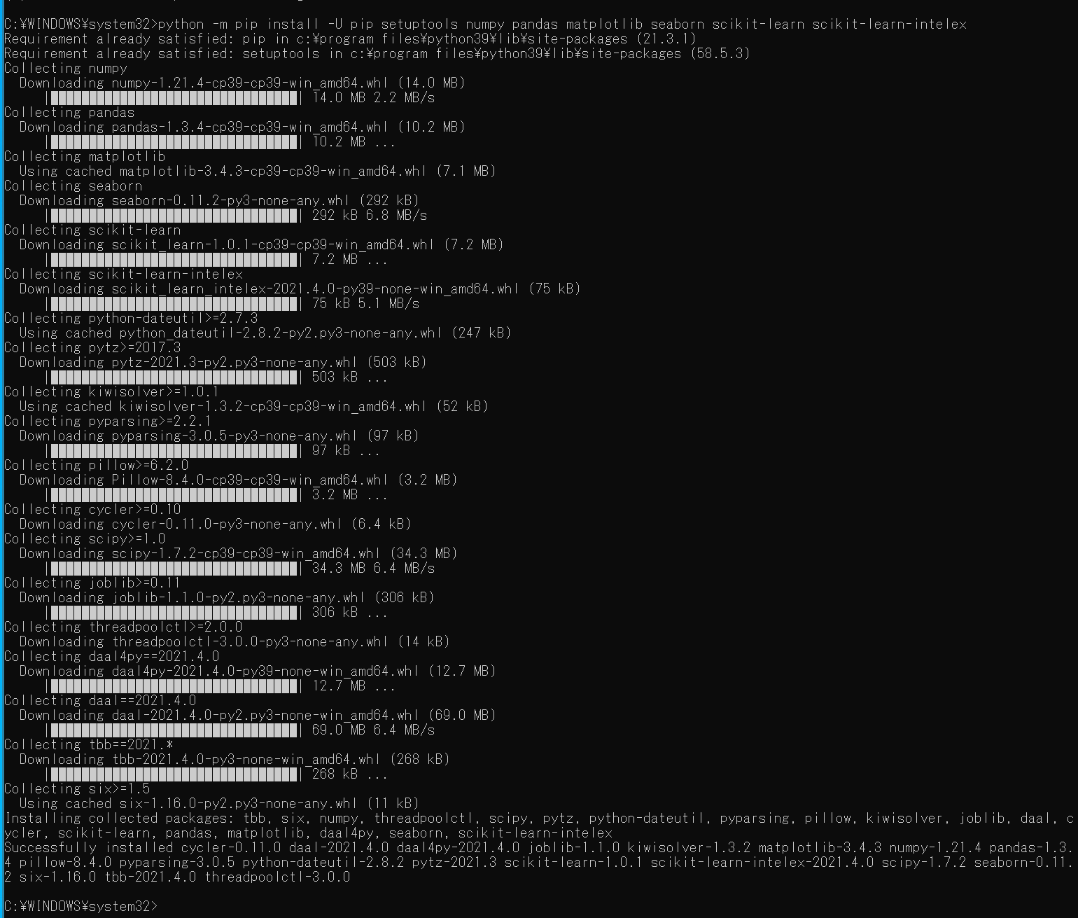
Windows では，コマンドプロンプトを 管理者として実行し，次のコマンドを実行する．
python -m pip install -U pip setuptools numpy pandas matplotlib seaborn scikit-learn scikit-learn-intelex

Ubuntu の場合

端末で，次のコマンドを実行

# パッケージリストの情報を更新
sudo apt update
sudo apt -y install python3-numpy python3-pandas python3-seaborn python3-matplotlib python3-sklearn

2. Iris データセット, titanic データセットの準備

iris, titanic データセットの読み込み

import pandas as pd
import seaborn as sns
sns.set()
iris = sns.load_dataset('iris')
titanic = sns.load_dataset('titanic')

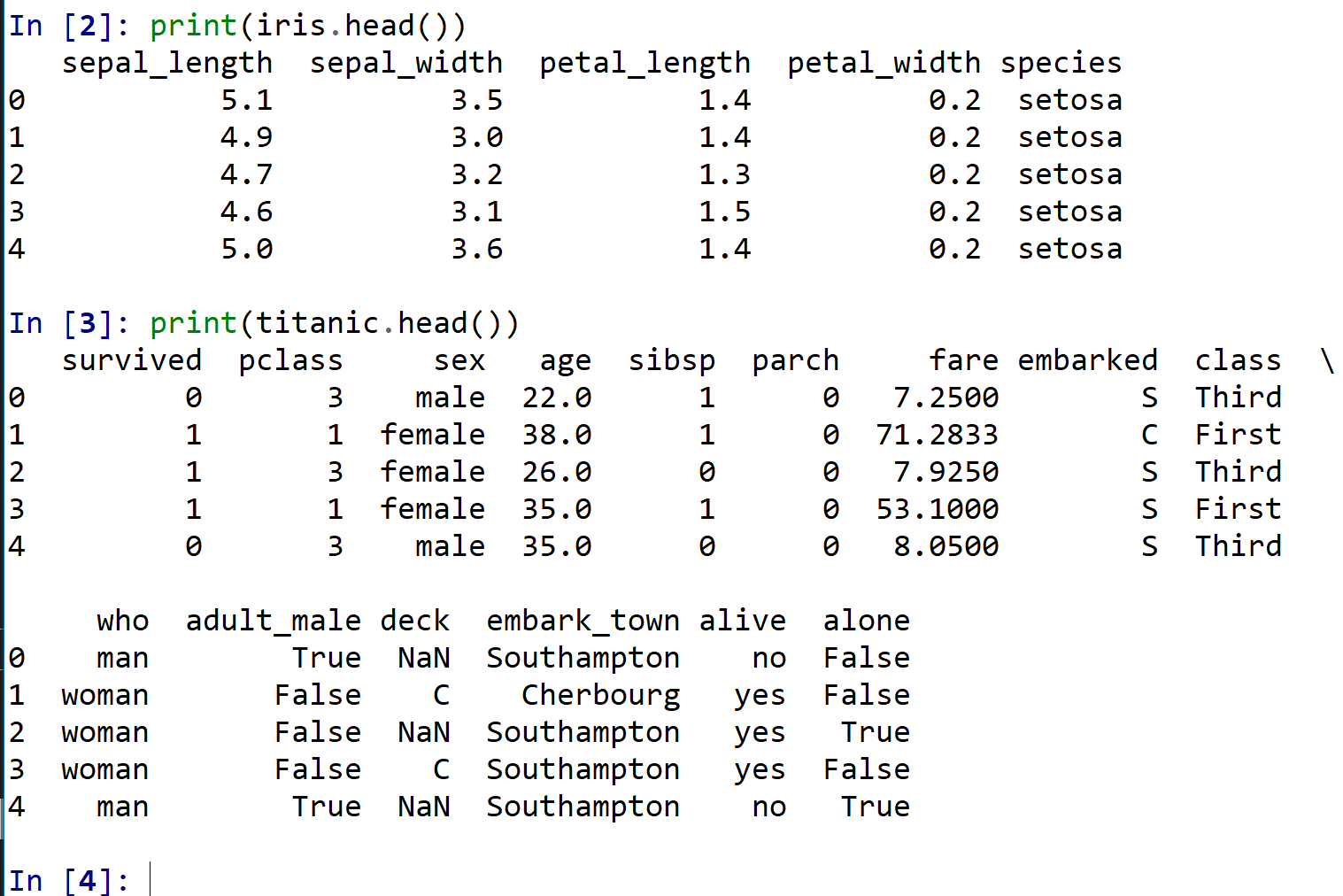
データの確認

print(iris.head())
print(titanic.head())

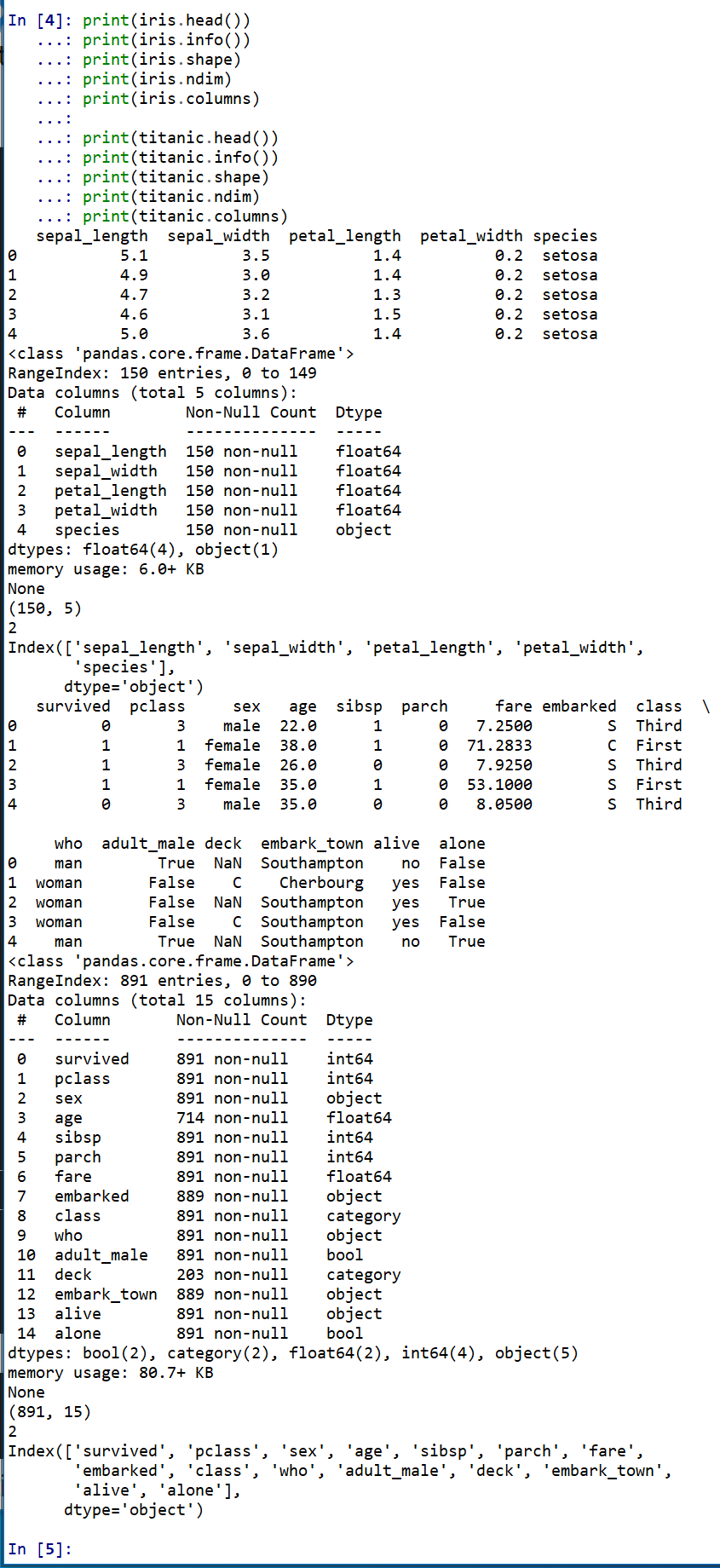
3. 基本的な情報の表示

head: 先頭部分の表示
shape: サイズ
ndim: 次元数
columns: 属性名
info(): 各属性のデータ型

print(iris.head())
print(iris.info())
print(iris.shape)
print(iris.ndim)
print(iris.columns)

print(titanic.head())
print(titanic.info())
print(titanic.shape)
print(titanic.ndim)
print(titanic.columns)

4. 散布図

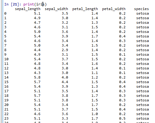
読み込んだ Iris データセットの表示
print(iris)
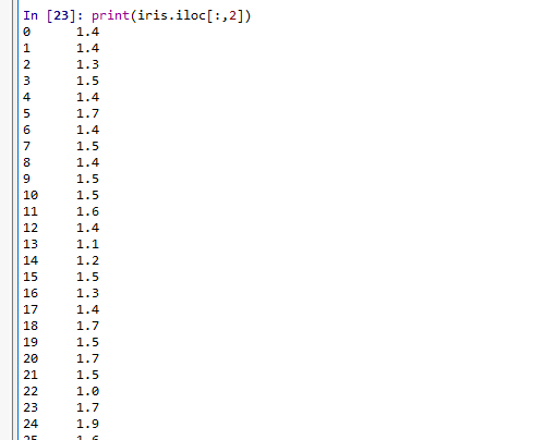
Iris データセットのうち、1列目と 2列目の表示
* オブジェクト iris には 0, 1, 2, 3, 4列目がある．
print(iris.iloc[:,1]) print(iris.iloc[:,2])

Iris データセットについて、1列目と 2列目の散布図

「plt.style.use('ggplot')」はグラフの書式の設定．「ro」は「赤い丸」という意味．

%matplotlib inline
import matplotlib.pyplot as plt
import warnings
warnings.filterwarnings('ignore')   # Suppress Matplotlib warnings
plt.style.use('ggplot')
plt.plot(iris.iloc[:,1], iris.iloc[:,2], 'ro')
plt.show()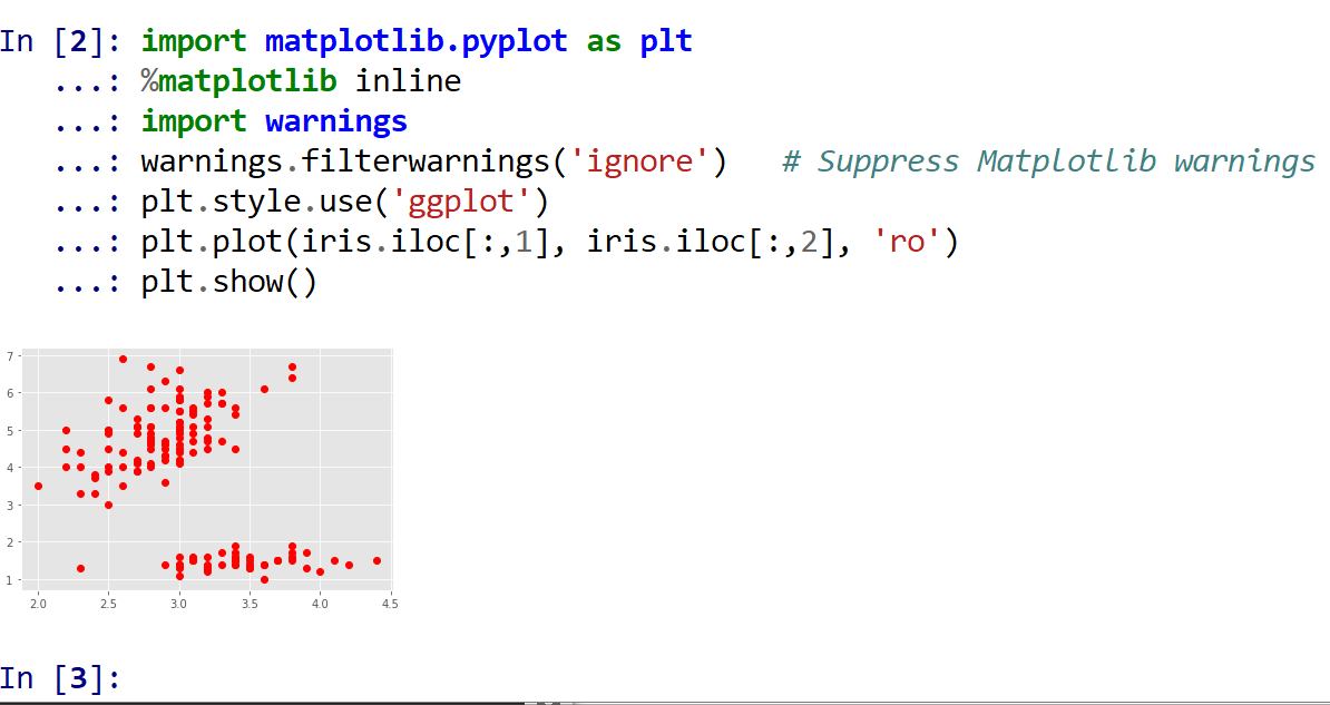

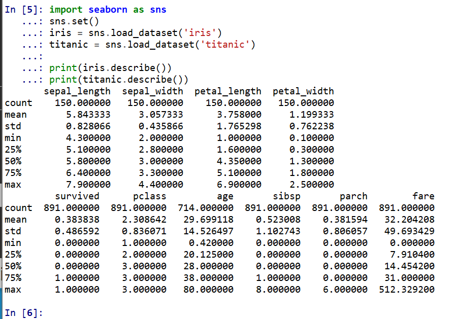
5. 各属性の要約統計量（総数、平均、標準偏差、最小、四分位点、中央値、最大）

import seaborn as sns
sns.set()
iris = sns.load_dataset('iris')
titanic = sns.load_dataset('titanic')

print(iris.describe())
print(titanic.describe())

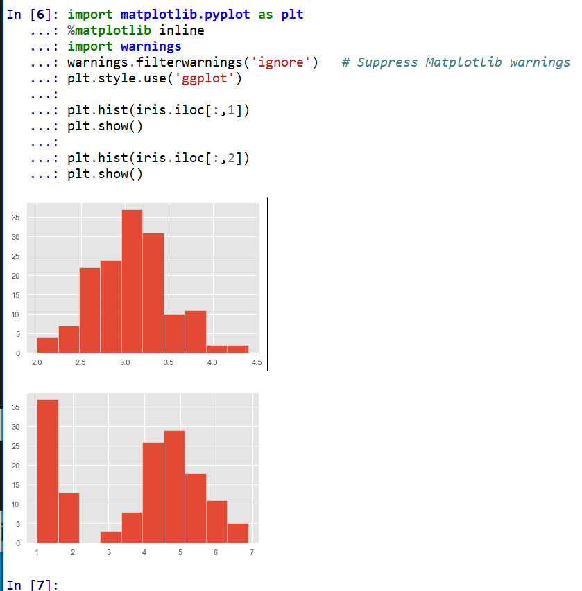
6. ヒストグラム

%matplotlib inline
import matplotlib.pyplot as plt
import warnings
warnings.filterwarnings('ignore')   # Suppress Matplotlib warnings
plt.style.use('ggplot')

plt.hist(iris.iloc[:,1])
plt.show()

plt.hist(iris.iloc[:,2])
plt.show()

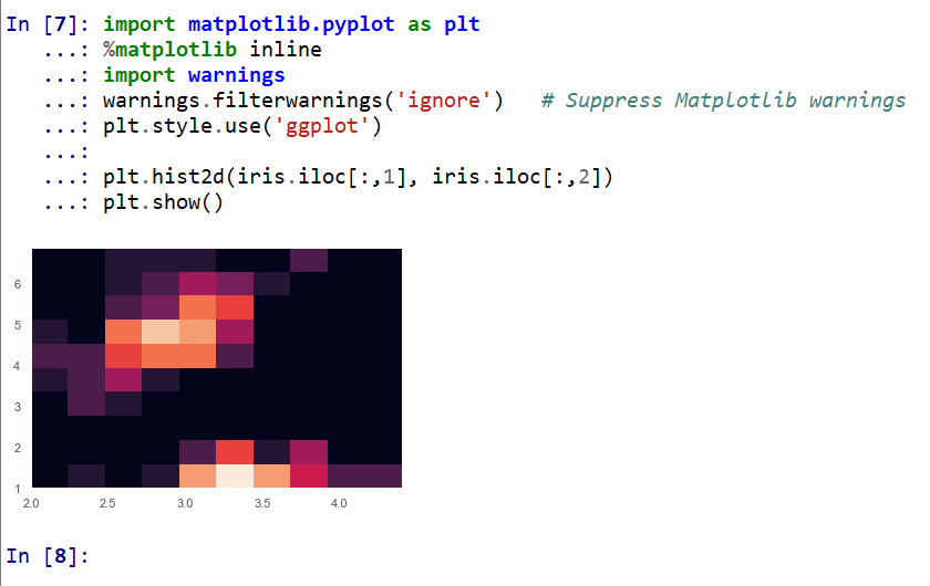
２次元ヒストグラム

%matplotlib inline
import matplotlib.pyplot as plt
import warnings
warnings.filterwarnings('ignore')   # Suppress Matplotlib warnings
plt.style.use('ggplot')

plt.hist2d(iris.iloc[:,1], iris.iloc[:,2])
plt.show()